
A Block Size Optimization Algorithm for Parallel Image Processing
J. Alvaro Fernández and M. Dolores Moreno
Dept. Ing. Eléctrica, Electrónica y Automática, Escuela de Ingenierías Industriales, Universidad de Extremadura,
Av. Elvas s/n, 06006, Badajoz, Spain
Keywords: Block Processing, Parallel Processing.
Abstract: The aim of this work is to define a strategy for rectangular block partitioning that can be adapted to the
number of available processing units in a parallel processing machine, regardless of the input data size.
With this motivation, an algorithm for optimal vector block partitioning is introduced and tested in a typical
parallel image application. The proposed algorithm provides a novel partition method that reduces data
sharing between blocks and maintains block sizes as equal as possible for any input size.
1 INTRODUCTION
It is a well-known fact that a series of image
processing operations usually involves a previous
partition of the image in sections, commonly
referred to as blocks, windows or neighbourhoods.
This is the case of many low-level operations, such
as linear filters, nonlinear processing filters like
local median and rank-order filters and local
histogram computing, to name a few (Bovik, 2005).
In the last decade, this Block Processing (BP)
paradigm has gained special significance after
multicore architectures had taken the lead as parallel
Processor Units (PUs), including embedded real-
time processors, FPGAs and GPUs (Bailey, 2011).
Parallel Image Processing (PIP) is probably the
only valid choice if a real-time response over high
resolution images is required. Given a number of
available PUs, a block partition for parallel BP
should be addressed in order to adapt the data to the
available processors.
Nowadays, specialized technical software like
MATLAB (Moler, 2007) and Mathematica
(Mangano, 2010) utilizes parallel processing
intensively. Both of them are used by many
researchers in the field of Digital Image Processing
(DIP).
But BP is also used in other disciplines –and
their associated software. This is the case of
statistical applications on Geographical Information
Systems (GIS), for which ArcGIS may be arguably
claimed to be the usual commercial software choice
(de Smith et al., 2013).
The ability of partition a series of data associated
with some topological 2D map enables local
statistical analyses via the so-called raster
operations.
In GIS, a raster or grid is a spatial (geographic)
data structure that divides a region into
neighbourhoods (or cells) that can store one or more
values for each of them, usually statistical data. A
raster is often contrasted with vector data, which is
used to represent points, lines and polygons.
The analogy between a raster and a digital image
is straightforward. In fact, most of the data collected
in a raster is usually represented with images of
some kind (de Smith et al., 2013).
In addition, this kind of scenario is well-suited to
be addressed by a set of PUs, which should be able
to work in parallel. Thus, a direct relationship
between topological partition and process
parallelization may be established.
The aim of this work is to devise a strategy for
data block partitioning (BP) that can be optimally
adapted to the number of available PUs, regardless
of the input data size. An optimal partition should be
able to provide minimum block size differences and
minimum –if any– overlap between adjacent blocks.
The paper is organized as follows. Section 2
reviews basic background for raster operations and
neighbourhood configurations for parallelized BP
techniques. Section 3 describes a novel algorithm for
partition an image into optimally similar area blocks
in order to be used by different PUs. Experimental
results are presented in Section 4. Finally, Section 5
concludes the paper.
138
Alvaro Fernandez J. and Dolores Moreno M..
A Block Size Optimization Algorithm for Parallel Image Processing.
DOI: 10.5220/0004695001380144
In Proceedings of the 9th International Conference on Computer Vision Theory and Applications (VISAPP-2014), pages 138-144
ISBN: 978-989-758-003-1
Copyright
c
2014 SCITEPRESS (Science and Technology Publications, Lda.)

Figure 1: Some neighbourhood shapes.
2 BACKGROUND
2.1 Raster Operations
Raster operations can be classified into three groups:
Local, where operations are performed in a
cell by cell fashion;
Neighbourhood, for which operations are
computed using a moving group of cells and
Zonal, where operations are performed using
groups of similar cells (zones).
In a local raster, an output cell
,
is
computed as a function of the corresponding input
cell
,
, i.e.
,
,
,
(1)
where is called a mapping or point operation over
input , which is independent of the cell position
,
and thus can be implemented as a look-up table
(LUT) (Bovik, 2005). In GIS, a local raster may be
used for data reclassification (de Smith et al., 2013).
In Digital Image Processing (DIP), a local raster
may be employed for thresholding a graylevel input
image.
A neighbourhood raster utilizes for each input
cell X(i,j) and its associated neighbourhood
,
,
the information of the cells belonging to the region
,
to determine the output cell value
,
via
a neighbourhood operation that –again– can be
modelled as a mapping function for which, in this
case,
,
,
.
(2)
This neighbourhood
,
is usually a region of
X centred around the input cell
,
, shaped as a
rectangle, but that can also be defined with other
shapes (see Fig. 1).
In this sense, it can be said that a local raster is
just a special case of a neighbourhood raster, for
which the neighbourhood
N
is constant for every
input cell
,
, being a rectangle of size 1×1.
A typical example of neighbourhood raster in DIP is
linear spatial filtering and nonlinear local filtering.
This approach is also utilized both in GIS and DIP
applications for computing local statistics of the
neighbours of a cell (or pixel).
Finally, a zonal raster operation involves groups
of cells –called zones– that present similar values.
Each one of these group can be considered to be a
connected group of cells or labels. Thus, a label is
defined as the group of cells for which a spatial
connectivity exists, i.e. any pixel inside the label can
be accessed from every other pixel in the same label
by following a spatial trajectory that does not fall
outside the label boundary at any step.
Typical label measurements are object perimeter
and area (Bovik, 2005), but they can also include
statistical information. In this context, a label can
also be thought of a special kind of neighbourhood,
which is topologically separated from the other
labels belonging to the zone.
2.2 Parallel Processing Techniques
Virtually all image processing techniques are based
on a sequence of image processing operations, i.e.
they are designed as a sequential algorithm or a
sequence of operations. This is a form of temporal
parallelism that can be exploited in a so-called
pipelined structure (Bailey, 2011).
In the pipeline depicted in Fig. 2, a separate PU
is used for each operation or task. The latency of an
image processing may be defined as the time
between when the first input is applied to the first
task of the pipeline and the corresponding output of
this data is available at the end of the pipeline.
Another example of pipeline is that of a buffered
video processor, in which each frame is processed
by the same group of techniques. Thus, the image
sequence may also be partitioned in time, by
assigning successive frames to separate processors,
leading to a hierarchical pipeline.
In general, the smaller the neighbourhood needed
to perform the operation, the lower its latency. Thus
a local raster has the lowest latency, whereas an
operation which needs every pixel in the image will
have the highest latency (Downton and Crooke,
1998).
Figure 2: A pipeline for temporal parallelism exploitation.
…PU
1
Operation 1
PU
N
Operation N
ABlockSizeOptimizationAlgorithmforParallelImageProcessing
139

Figure 3: Spatial parallelism exploitation by block
partitioning (BP): row, column and rectangular BP.
However, as the algorithm increases its
complexity, the operation pipeline speedup becomes
less important, mainly due to operation
hierarchization and feedback. In this case, the major
speedup may be obtained within a specific operation
in the form of loops.
The outermost loop within each operation
usually iterates over the pixels within the image,
because many operations (e.g. spatial filtering)
perform the same function independently on many
pixels.
This is spatial parallelism, which may be
exploited by partitioning the image and using a
separate processor to perform the operation on each
partition (Bailey, 2011).
2.3 Block Partition Schemes
An important consideration when partitioning an
image is to minimize the expected communication
between PUs, i.e. between the different considered
partitions.
Typical partitioning schemes split the image into
blocks of rows, blocks of columns or rectangular
blocks, as illustrated in Fig. 3.
For low-level DIP operations such as spatial
filtering, the performance improvement approaches
the number of processors, as the communication
may be reduced to zero if a non-overlapping
partition scheme is utilized.
However, in higher level processes this
performance will be degraded as a result of
communication overheads or contention when
accessing shared resources. In high-level operations,
these shared resources may just not be pixel values.
Partitioning is therefore most beneficial when the
operations only require data from within a local
region, which is defined by the partition boundaries.
For that reason, each processor must have some
local memory to reduce any delays associated with
contention for global memory (Bailey, 2011).
If the operations performed within each region
are identical, this leads to a SIMD (single
instruction, multiple data) parallel processing
architecture.
On the other hand, a MIMD (multiple instructions,
multiple data) architecture is better suited for higher
level image operations, where latency may vary for
each block of data.
In these cases, better performances may be
achieved by having more partitions than processors,
utilizing a Pipeline Processor Farm (PPF) approach
(Fleury and Downton, 2001). In a PPF, each
partition is dynamically allocated to the next
available PU, thus reducing idle process latencies
related to block data dependencies.
In the next section, a procedure for block
partitioning will be devised to be optimally suited to
a PPF approach.
3 AN ADAPTIVE BLOCK
PARTITIONING PROCEDURE
3.1 Overlapping Neighbourhoods
Rectangular block partitioning is by far the main
shape choice in low-level image operations (Davies,
2012). Two types of rectangular neighbourhoods are
commonly considered: overlapping and non-
overlapping.
In spatial linear filtering, a series of sums and
products are needed for each pixel within the input
image, with pixels, as a result of applying a
small kernel of weight elements over the pixel
surrounding neighbours. In this case, each pixel and
its neighbourhood can be processed by a single PU
and no inter-process communication is needed.
Except for the border pixels of the image, where
additional data –usually zero values– is needed to
complete the neighbourhood, each PU can read the
corresponding pixel information directly from the
image and return its own data as output.
This same concept applies to focal statistics (de
Smith et al., 2013), where a neighbourhood raster is
applied. The algorithm visits each cell in the raster
and calculates a specific statistic over the identified
neighbourhood. As neighbourhoods can overlap,
cells in one neighbourhood will also be included in
any neighbouring cell’s neighbourhood.
This situation may enable data reutilization in the
raster (Huang et al., 1979), thus reducing shared
memory accesses in a PPF environment.
On the other hand, non-overlapping partitions
may be used for parallelization speedup in
hierarchical parallel schemes. This paradigm is best
suited for distributed memory MIMD architectures,
in which each PU handles its own local memory
VISAPP2014-InternationalConferenceonComputerVisionTheoryandApplications
140

(Fleury and Downton, 2001).
In DIP, non-overlapping block processing is
widely used in applications such as image scaling
(e.g. image pyramids), compression (e.g. DCT
computing) and recognition (e.g. ridge orientation
assessment in fingerprint representation) (Ratha et
al., 1996).
In GIS applications, this approach is also known
as block statistics. In block statistics, the algorithm
performs a neighbourhood raster that calculates a
statistic for input cells within a fixed set of non-
overlapping neighbourhoods.
The statistic (e.g. dynamic range, average or
sum) is calculated for all input cells contained within
each neighbourhood. The resulting value for an
individual neighbourhood or block is assigned to all
of its cell locations.
Since the neighbourhoods do not overlap, any
particular cell will be included in the calculations for
only one block. In other words, distributed parallel
computation of each block is possible with no
further cost.
Somewhere between these two methods, a small
overlap between adjacent neighbourhoods is also
used in several DIP techniques, such as (Kuwahara
et al., 1976). This approach is a trade-off between
the fully overlapping and non-overlapping
neighbourhood paradigms, which enables the user to
control the speedup with the aid of an overlap factor.
With a controlled neighbourhood overlap, a
raster may estimate a particular statistic by
performing a smaller amount of calculations, with
the cost of a later interpolation stage (Davies, 2012).
In addition, this approach shares the benefits and
drawbacks of both overlapping and non-overlapping
PPF design.
3.2 Definitions
3.2.1 Rectangular Neighbourhood
For a particular input cell or pixel located at
,
within a discrete digital input
X
, a rectangular
neighbourhood
of size may be defined as
the set
,
,
,
(3)
for which
max
|
|
and max
|
|
,
(4)
where and are positive integers that set the
vertical and horizontal radius of the neighbourhood
around the central position
,
, respectively. Thus,
a pixel neighbourhood
yields a 3×5 rectangular
block of input cells.
Figure 4: Complete vector partitions (top to bottom):
regular non-overlapping, regular fixed overlapping,
irregular non-overlapping, irregular fixed overlapping,
irregular loose overlapping and regular loose overlapping.
3.2.2 Vector Partitions
Let ̅ be a single-dimensional discrete vector of
length . A partition of ̅ into non-empty parts,
̅,
, may be defined as a group of subsets ̅
of
̅, i.e.
̅,
̅
for 0, where each part
̅
is a subset of ̅ of length
, with the following
property:
Given any two elements of ̅
with vector
positions
and
, where 0
and
their corresponding positions in ̅,
and
, with
0
, the following condition is hold:
.
(5)
In other words, each part ̅
keeps the original
relative positions of their elements in ̅ and no
element of ̅ is missed between the first and the last
element in any part ̅
.
A partition
̅,
is said to be complete if and
only if (iff) the set union of all the parts of ̅ yields
̅, i.e. iff
⋃
̅
̅. Otherwise, it is said to be
incomplete. From this point on, our discussion will
only deal with complete partitions.
Table 1: Vector Partition Types.
Type Condition
Regular
,∀,
Pseudo-regular
max
1,∀,
Fixed
0
,∀,
Tight
max
1,∀,
In a complete partition, every element of ̅
belongs to at least one of its parts. In Fig. 4 a series
of six different complete vector partitions is
illustrated.
A complete partition
̅,
is said to be regular
iff each part ̅
has the same length, i.e. iff
ABlockSizeOptimizationAlgorithmforParallelImageProcessing
141

,∀,. Thus, in this case
. Otherwise, the
partition is called irregular. In Fig. 4, the first,
second and sixth partitions are regular.
A special case of irregular partition is also of
interest. A pseudo-regular partition
̅,
is an
irregular complete partition whose different part
lengths obey the following expression:
max
1,∀,
.
(6)
A complete partition
̅,
is said to be non-
overlapping iff the set intersection of any two parts
of ̅ is the empty set, i.e. iff ̅
∩̅
∅,∀.
Otherwise, it is called overlapping. In Fig. 4,
overlapping partitions are depicted with their
overlapping parts shaded.
An overlapping partition
̅,
may, of course,
be regular iff
,∀,. However, if the overlap
sections shared between two adjacent parts ̅
and
̅
, for 0 , have constant size
0, the
overlapping partition is said to be fixed, i.e. if
0
,∀,. Otherwise, it is said to be loose.
Both second and fourth partitions illustrated in Fig. 4
are fixed.
An overlapping fixed partition may be
represented with the special notation
̅,,
,
where its main parameters, , and are positive
integers bound to the equation
1
,
(7)
where
∑
is called the limit length of the
partition, i.e. the accumulated length of its parts. In
addition, if
and 1, then the positive
condition for is always met,
0.
(8)
Finally, a special kind of overlapping partition is
also considered. A tight overlapping partition
̅,
is a loose overlapping partition whose
different overlap section sizes
follow the relation
max
1,∀,
. (9)
For convenience, a summary of the previous
definitions is collected in Table 1.
3.3 A Vector Partition Algorithm for
Parallel Block Processing
Given an input vector ̅ and a fixed part size , an
optimal partition
̅,
is sought. The optimality
of the partition is based on the discussion of Sections
2.2 and 2.3, where a PPF is supposed to be used to
perform some operation over the input vector. Thus,
our main interests are: 1) to keep partition parts as
equal in size as possible and 2) to reduce
overlapping to a minimum.
Moreover, the optimal partition selection
algorithm will be performed as follows:
First, if a regular non-overlapping partition
exists, it will be chosen as optimal;
Otherwise, if a non-overlapping pseudo-
regular partition is possible, it will be chosen
in the second place,
Third, if none of the above possibilities are
available, an overlapping fixed partition will
be selected, with the minimum amount of
overlap.
From the previous section, we know that if
/ is a positive integer 0, then
̅,
will
be a regular non-overlapping partition.
However, for this preferred case to occur, must
be an integer divisor of and must not be prime.
Otherwise, a pseudo-regular partition should be
chosen.
The following algorithm is proposed for
obtaining a non-overlapping pseudo-regular partition
̅,
of elements with fixed part length, :
Let mod, with 0.
If 1/2,
Let
/
,
and
1.
Else
Let
/
,
and
1.
End
In the previous algorithm, the number of parts
of the partition is defined such that the number of
pseudo-parts
of length
is minimal and
condition (6) is maintained. Thus, a pseudo-regular
partition
̅,
is obtained.
However, the specific distribution of the
pseudo-parts still remains undefined. Between all the
possibilities, a symmetric distribution with maximal
distance between pseudo-parts is proposed. This
kind of distribution should enable the best balance of
any possible side effect as a result of the pseudo-
regular kind of the partition.
Let be a
-elements vector of pseudo-part
positions
∈
0,
,∀ in
̅,
. A
symmetric distribution of the pseudo-parts in a
pseudo-regular non-overlapping partition can be
obtained with the following algorithm:
If
is odd,
Let
/2
/2
.
End
If
1,
Let /
1
with 1.
For 0to
/2
VISAPP2014-InternationalConferenceonComputerVisionTheoryandApplications
142
Let
,
1.
End
End
Thus, if the number of pseudo-parts is odd, one
of them should be the central part of the partition. In
addition, each pseudo-part would be separated by
parts, including the first and last parts of
̅,
.
The previous algorithm would only yield pseudo-
regular non-overlapping partitions iff 1.
Otherwise, the obtained partition cannot ensure
optimal criteria (e.g. block pseudo-regularity).
In these cases, a third kind of partition should be
chosen. This new partition scheme should have, at
least, pseudo-regular overlapping parts with fixed
overlap .
With the aid of (7), it is possible to apply the
previous algorithm to a new non-overlapping
partition with length equivalent to the limit length
of an overlapping fixed partition
̅,,
, for
increasing . Once the equivalent pseudo-regular
partition is obtained, a fixed overlap is performed in
each of its parts.
3.4 N-D Block Partitions
The optimal vector partition algorithm discussed in
Section 3.3 may be separately applied to each
dimension of a n-D discrete input data.
In this case, the obtained n-D partition is called a
n-D block partition (BP).
Table 2: 16-element Vector complete Partitions.
1 16 0 0 16
2 8 0 0 16
3 6 2 0 16
4
4
0 0 16
5
3
1 0 16
6
3
2 0 16
7
2
2 0 16
8
2
0 0 16
9
2
2 0 16
10
2
0 4 20
11
2
0 6 22
12
2
0 8 24
13
2
0 10 26
14
2
0 12 28
15
2
0 14 30
16
1
0 0 16
4 PARTITIONING EXAMPLES
In the first example, the optimal partition algorithm
of Section 3.3 is applied to a vector with 16
elements. The algorithm is executed for part lengths
with 1,2,…,. The resulting partitions are
presented in Table 2. Not until a relatively large part
size, 10, the algorithm delivers an overlapping
partition as optimal. From this part length on, two
overlapping parts are set as the optimal partition for
the test vector with minimum overlap v.
In the second test, two optimal partitions for a
block decimation colour scale pyramid are computed
for Lena image, of 512×512 px. The chosen
decimation factors for this example are 1/15 and
1/25, thus block partitions for = 15 and = 25 are
computed using the algorithm of Section 3.3.
Clearly, neither 15 nor 25 are integer divisors of
512. Thus, the obtained optimal partitions are both
pseudo-regular non-overlapping, as depicted in Fig.
5. These partitions are optimal as they yield
minimum overlap and minimum amount of blocks
with different lengths. In this case,
= 2 for = 15
and
= 13 for = 25.
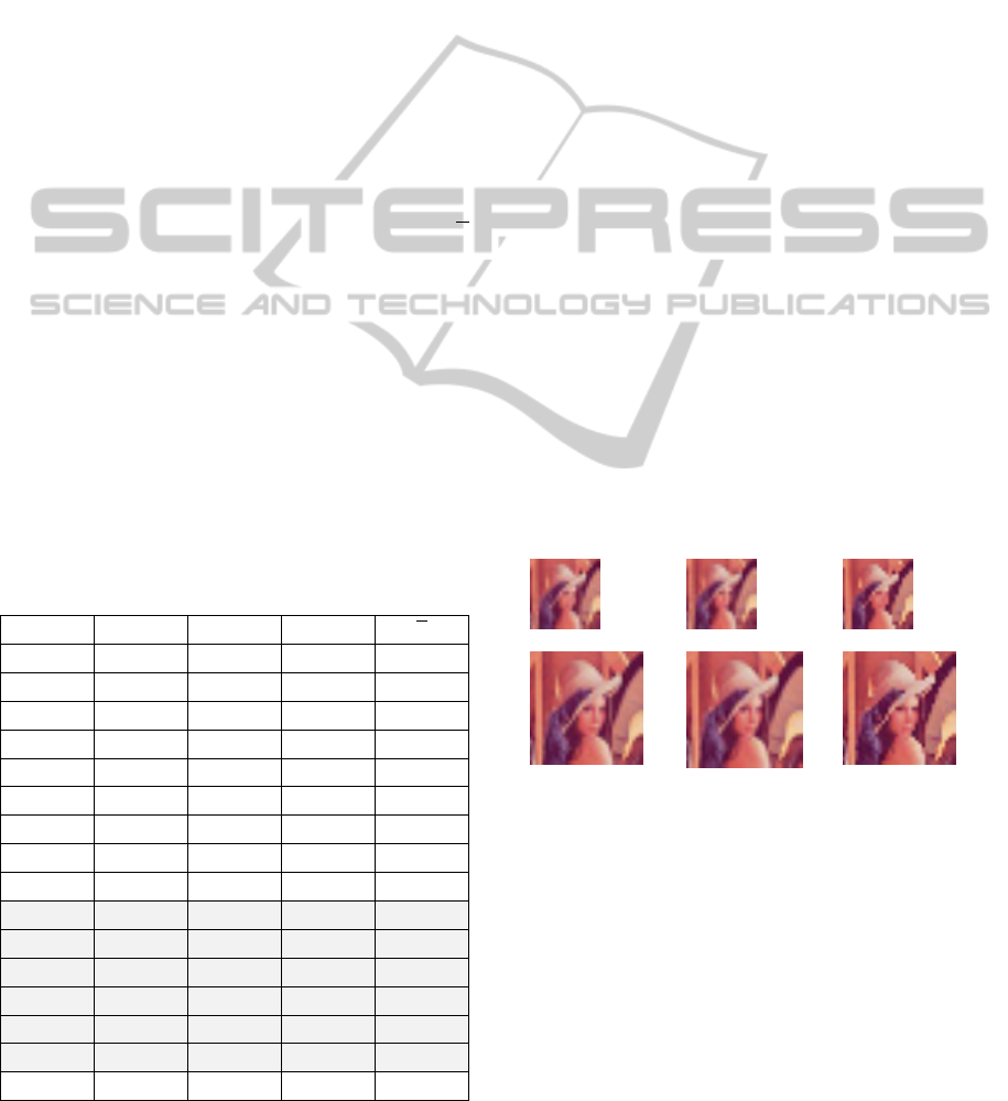
In Fig. 6, the resulting output decimated block
images are displayed. Both local mean and median
are used for computing each pixel in the decimated
image. For reference purposes, an additional
bicubic-decimated image is also shown in Fig. 6.
This latter filter is not based on the proposed optimal
blocks.
a. b. c.
Figure 6: 1/25 and 1/15 block decimation for Lena (2x
scale): a) block mean, b) bicubic interpolation and c) block
median.
5 CONCLUSIONS
In this paper, a vector partition algorithm with
applications in parallel processing environments,
such as PPF, has been introduced.
From a theoretical discussion on the description
and classification of vector partitions, which can be
ABlockSizeOptimizationAlgorithmforParallelImageProcessing
143

a.
b.
Figure 5: Optimal block partitions for Lena: a) = 25 and
b) = 15.
extended to the n-dimensional case, the application
of the proposed algorithm has been tested on a
typical image decimation stage.
The algorithm produces a block partition which
is optimized to be processed in PPF frameworks.
The proposed optimization procedure focuses in
both minimizing possible size differences in process
loads, and maintaining inter-block data sharing at a
minimum, by selecting the minimum amount of
overlap between adjacent blocks.
In combination with time parallelization,
possible applications of the proposed algorithm in
real-time processing platforms may accelerate some
common high load pre-processing tasks in computer
vision, such as statistical analysis from local
histograms.
In a parallel processing machine, the proposed
algorithm should enable a BP scheme which may be
real-time adapted to the instantaneous availability of
PUs in the environment.
ACKNOWLEDGEMENTS
This work has been supported by the Regional
Government of Extremadura through the European
Regional Development Fund (GR10097). The
authors would also like to thank the anonymous
reviewers for their valuable comments and
suggestions to improve the quality of the paper.
REFERENCES
Bailey, D. G., 2011. Design for Embedded Image
Processing on FPGAs. Wiley. Singapore, Singapore.
Bovik, A. (ed), 2005. Handbook of Image and Video
Processing, 2
nd
ed. Academic Press, London, UK.
Davies, E. R., 2012. Computer and Machine Vision:
Theory, Algorithms, Practicalities, 4
th
ed. Academic
Press, Oxford, UK.
de Smith, M. J., Goodchild, M. F., Longley, P. A., 2013.
Geospatial Analysis: A Comprehensive Guide to
Principles, Techniques and Software Tools, 4
th
ed, The
Winchelsea Press. Winchelsea, UK, www:
http://www.spatialanalysisonline.com.
Downton, A., Crookes, D., 1998. Parallel Architectures for
Image Processing, Electronics and Comm Eng J,
10(3), pp. 139-151, doi: 10.1049/ecej:199803072010.
Fleury, M., Downton, A., 2001. Parallel Processing
Farms: Structured Design for Embedded Parallel
Systems. Wiley. Singapore, Singapore.
Huang, T. S., Yang, G. J., Tang, G. Y, 1979. A Fast Two-
Dimensional Median Filtering Algorithm. IEEE Trans
Acoustics Speech Signal Proc, 27(1), pp. 13-18, doi:
10.1109/TASSP.1979.1163188.
Kuwahara, M., Hachimura, K., Ehiu, S., Kinoshita, M.,
1976. Processing of Ri-Angiocardiographic Images, in
Preston, K., Onoe, M. (eds). Digital Processing of
Biomedical Images, Plenum Press, pp. 187-202, New
York, USA, doi: 10.1007/978-1-4684-0769-3_13.
Mangano, S., 2010. Mathematica Cookbook. O’Reilly.
Sebastopol, USA.
Moler, C., 2007. Parallel MATLAB: Multiple Processors
and Multiple Cores, The Mathworks News & Notes,
www: http://www.mathworks.com/tagteam/42682_
91467v00_NNR_Cleve_US.pdf.
Ratha, N., Karu, K., Chen, S., Jain, A., 1996. A Real-Time
Matching System for Large Fingerprint Database,
IEEE Trans Pattern Anal Machine Intell (PAMI),
18(8), pp. 799-813, doi: 10.1109/34.531800.
VISAPP2014-InternationalConferenceonComputerVisionTheoryandApplications
144
