
Tone Mapping for Single-shot HDR Imaging
Johannes Herwig, Matthias Sobczyk and Josef Pauli
Intelligent Systems Group, University of Duisburg-Essen, Bismarckstr. 90, 47057 Duisburg, Germany
Keywords:
High Dynamic Range Imaging, Tone-reproduction Operators, Noise Reduction, Image Segmentation.
Abstract:
The problem of tone mapping for HDR (high dynamic range) to LDR (low dynamic range) conversion is
introduced by a unified framework considering all the usual processing steps. Then the specific problem of
single-shot HDR is outlined where special emphasis is taken on the effect of the greater noise floor of those
images when compared to the usual exposure bracketing approach to HDR. We herein tailor the popular tone
mapping operators proposed by Reinhard for single-shot HDR. A region-based approach for preprocessing
any HDR image in order to increase SNR and perceptual sharpness is introduced as an extension to our initial
tone mapping framework. The results are compared with respect to specially developed baseline tone mappers
and an extensive subjective evaluation is performed.
1 INTRODUCTION
Tone mapping operators are used in a high dynamic
range (HDR) image acquisition and processing chain
(Reinhard et al., 2010) as the final completion. Tone
mapping allows displaying or printing a HDR image
on LDR (low dynamic range) media by compressing
the wide tonal range of the HDR image into an im-
age with lower tonal sampling. Thereby the bit-depth
of the HDR image pixel commonly is 32-bit floating
point but LDR images are only 8-bit unsigned inte-
gers. Tonal compression should be able to preserve
the overall contrast, textural details and color fidelity
of the original image (Frazor and Geisler, 2006).
Often only a HDR image is capable of captur-
ing the real dynamic range of any natural scene, but
both consumer digital displays and printing technolo-
gies are only capable of dealing with low dynamic
range images (DiCarlo and Wandell, 2000). The crux
thereby is that photographers usually want to create
a ”true” reflection of their visual experiences which
they want to convey to their viewers, but due to lim-
ited capturing and displaying technologies any photo-
graph can never be as visually rich as the real scene.
Therefore, the tone mapper is crucial in delivering
an image that ”feels” as naturalistic as possible when
viewed at low dynamic range.
Although, tone mapping operators are developed
with the (in-)capabilities of the human visual system
(HVS) in mind, their design can be considered more
an art than engineering. This is also because of the
vast amount of factors that influence the sensation of
an image where lots of assumptions are to be made.
For example, apart from the tonal richness of the par-
ticular HDR image additional properties of the view-
ing conditions and the audience are to be considered:
specific display technology, viewing distance, ambi-
ent lighting, emotional state, cultural background, etc
(Bodrogi and Khanh, 2012).
In this paper, we present several extensions and
enhancements of the tone mapper for photographic
tone reproduction originally introduced by Reinhard
(Reinhard et al., 2002). Reinhard has developed dif-
ferent tone mapping operators in the past which are
commonly acknowledged for their naturalistic results
thereby advancing this field of research (Reinhard
et al., 2010). His and other operators usually assume
that the HDR image was created by fusing a series of
differently exposed LDR images of the same scene.
1.1 Tone Mapping for Single-shot HDR
In our application scenario only one image is taken
with a pixel depth of 12-bit unsigned integer, which
means there are 4096 different values that we want
to tone map to 8-bit or 256 different values per color
channel. We use the so-called RAW imaging mode
of a digital camera which directly stores the raw but
color balanced pixels from the digital imaging sensor.
For our tone mapping we exploit the fact that mod-
ern digital consumer cameras internally have higher
analog-to-digital conversion (ADC) capabilities than
145
Herwig J., Sobczyk M. and Pauli J..
Tone Mapping for Single-shot HDR Imaging.
DOI: 10.5220/0004695401450152
In Proceedings of the 9th International Conference on Computer Vision Theory and Applications (VISAPP-2014), pages 145-152
ISBN: 978-989-758-003-1
Copyright
c
2014 SCITEPRESS (Science and Technology Publications, Lda.)

HDR image
Scaling of
channels
[0-1]
Create
luminance
image
Modify
tonal range
Normalize
tonal range
[0-1]
Gamma
correction
(γ)
Color
reproduction
Mapping to
target range
LDR image
Tone mapping operator
Color information
Brightness information
Figure 1: General framework for tone mapping.
their low dynamic range JPEG output images. This
ultimately means that these cameras already have im-
plemented proprietary tone compression algorithms.
These are however restricted to the light processing
power of current imaging processors and therefore
cannot perform advanced computations. In our ex-
perience the qualitative results of these global tone
mappers generally come close to some sort of gamma
correction which is one of the simplest tone mappers
and does not sufficiently lighten up shadowed parts
and tends to wash out textural details in brighter parts
of the image. Our globally and locally adaptive ap-
proaches are designed to overcome these issues.
The single-shot HDR approach provides a lower
dynamic range than real HDR capture using multiple
exposures. It however is easier to apply to dynamic
scenes. On the other hand, a single-shot HDR im-
age is noisier because there is no averaging of mul-
tiple exposures and since tone mappers are designed
for compressing wider dynamic ranges than a single
shot provides the noise tends to be intensified because
its is assumed to represent textural detail.
Although there are lots of different tone mapping
algorithms these nevertheless can be described by the
framework depicted in figure 1. Note that we always
perform an additional gamma correction after tonal
compression in order to comply with the usual ITU −
RBT.709 HDTV-standard for displaying devices.
2 PREVIOUS WORK
2.1 Linear Mapping
With a linear mapping a given range of values is
mapped to some target range by scaling with a con-
stant factor. HDR images that are downscaled this
way generally appear too dark and textural details in
shadowed regions get lost. This can be accommo-
dated by pre-scaling the HDR image like this:
I
0
(y, x) =
I(y, x) − I
mincut
I
maxcut
− I
mincut
with I
maxcut
, I
mincut
∈ {v | v ∈ R ∧ 0 < v ≤ 1},
I
maxcut
> I
mincut
, I(y, x) ∈ {0.0, . . . , 1.0} and intensities
I
0
(y, x) > 1.0 and I
0
(y, x) < 0.0 will get clipped.
I
maxcut
could be set in such a way that e.g. the up-
per 5% of intensities of the HDR image get clipped,
i.e. are collectively set to the maximum value of the
target range. This will result in a brightened LDR im-
age because fewer higher intensity outliers have less
impact on the overall scaling factor. Although the re-
sulting effect of burning pixels within highly lit image
regions causes lost textural details, it is positive for
perception (Reinhard et al., 2010) and enhances the
overall image contrast. We experimentally found that
clipping the higher 1% of intensities does not result in
any visually perceivable loss of information.
I
mincut
can be either set to zero or it can be sim-
ilarily used in order to clip the noise within darker
regions of the image which is especially useful for
single-shot HDR and further contributes to preserv-
ing visually important textural details in the resulting
LDR image. Thus I
mincut
could be set to the estimated
noise level (Immerkær, 1996) of the HDR image.
2.2 Global Photographic Mapping
Reinhard has successfully introduced an operator
(Reinhard et al., 2002) that is inspired by the zone
system of the famous photographer Ansel Adams.
A zone system splits the tonal range of the HDR
image into 11 different tonal zones from pure black
(zone 0) to pure white (zone 10). Zones 1 − 9 have
pre-set brightnesses which linearly blend into each
other. Thus zone 5 is of medium brightness and the
so-called scene key α maps to this zone. If α is
of relatively low brightness, then the overall image
is brightened up so that shadowed regions are better
visible but lighter regions loose richness at the same
time. If α is of relatively high brightness, then shad-
owed regions fully loose detail but brighter image re-
gions feature more textural richness.
This zone system is realized by the following tonal
compression of the normalized luminance image I:
I
0
(y, x) =
L
α
(y, x)
1 + L
α
(y, x)
·
1 +
L(y, x)
I
maxcut
(y, x)
2
whereby L
α
(y, x) denotes the intensity I(y, x) which is
scaled by the scene key α:
L
α
(y, x) =
α
I
avg
· I(y, x)
with α ∈ {x | x ∈ R ∧ 0 ≤ x ≤ 1} that can automat-
ically be computed (Reinhard, 2002) from the loga-
VISAPP2014-InternationalConferenceonComputerVisionTheoryandApplications
146

rithmic average I
avg
of the HDR luminance image as
α = 0.18 · 4
2·log
2
(I
avg
)−log
2
(I
mincut
)−log
2
(I
maxcut
)
log
2
(I
maxcut
)−log
2
(I
mincut
)
.
2.3 Local Photographic Mapping
Based on the global tone mapping operator presented
in the previous paragraph, a localized version of this
operator is given in (Reinhard, 2002). This oper-
ator is inspired by the technique of ”dodging and
burning” that has also been originally developed by
Ansel Adams when making photographic prints on
paper that were not straightforwardly capable of the
full tonal range of his film negatives. Here, every
pixel is selectively brightened up or darkened based
on an adaptively computed local neighborhood of
small enough intensity variance. Darker pixels that
are comprised by similar but somewhat lighter pixels
are damped more strongly than bright pixels that are
surrounded by relatively darker pixels, thereby creat-
ing higher local contrast in the tone mapped result.
This outlined the overall idea, but for more details the
reader is referred to Reinhard’s original publication.
3 PROPOSED APPROACHES
Based on the well-accepted algorithms of Reinhard
we propose the following extensions and enhance-
ments for single-shot HDR imaging.
3.1 Dynamic Scene Key
We present here the global photographic mapping
with a dynamic scene key α(y, x) that is different for
every image pixel. In the original algorithm α can
only be varied for the whole image, whereby an in-
creased α brightens the mid-tones but a decreased α
darkens the the whole image.
For improving the overall perception of image
contrast and simultaneously preserving or enhancing
local textural details it is only necessary to selectively
brighten up shadowed image regions but largely pre-
serve the local brightnesses of already bright image
regions in order to avoid the loss of visual detail. This
desired qualitative behavior of our proposed function
for computing α(y, x) is depicted by figure 2. Only
very bright intensities are starkly dampened and also
very dark intensities are smoothly cut-off since these
often tend to represent image noise. We experimen-
tally found the following adaptive α(y, x) which varies
with pixel intensity I(y, x):
α(y, x) = 1 − exp(−(I(y, x) · (1 + d · I(y, x)))
1−(I
avg
)
1
c
)
0
0.2
0.4
0.6
0.8
1
0
0.2
0.4
0.6
0.8
1
0
0.2
0.4
0.6
0.8
I(y, x)
I
avg
α(y, x)
Figure 2: The qualitative behavior of our varying scene key
α(y, x) with recommended c = 4. For better visualization
variable d is constantly set to 1 here.
with the user defined c ∈ {x | x ∈ N ∧ x > 0} and
d =
−1 if I(y, x) < I
avg
,
1 if I(y, x) ≥ I
avg
.
The constant c determines the overall strength
of the contrast enhancement. Thereby smaller val-
ues create greater contrast as is depicted in figure 3.
Note that only the shadowed image regions are starkly
brightened up with increasing c but that already bright
image regions are only moderately brightened which
works out as expected. This property makes the only
user parameter for computing α(y, x) to be robust for
a large amount of different scenes.
In our experiments a value c = 4 has been proven
to produce pleasing results for most scenes. For dif-
ferent scenes with an overall dark appearance the re-
sulting α is always between ≈ 0.63 and ≈ 0.86, but
for scenes with higher average brightnesses it usually
lies between ≈ 0.63 and ≈ 0.65.
3.2 Modified Local Photographic
For single-shot HDR we experienced that Reinhard’s
local photographic tone mapper can be safely used
with its default parameters because the comparatively
low dynamic range of RAW camera images does not
take advantage of those. Also shadowed regions are
adequately brightened up.
But we found that there is severe burning-in
among brighter parts of the scenes which causes su-
perfluous loss of detail and local contrast. Here we did
not change the original operator itself but the method
for normalizing the tonal range which is the first post-
processing step as depicted in figure 1. Here the stan-
dard method is to simply cut-off values I
0
(y, x) > 1.0.
After tonal compression, we propose to project all
the values I
0
(y, x) which are out of range into the valid
ToneMappingforSingle-shotHDRImaging
147
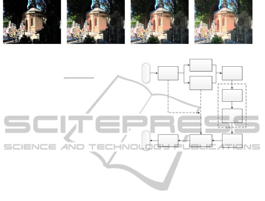
Figure 3: This image series shows the effect of parameter c (= 1, 4, 6 and 11) of the dynamic scene key α(y, x).
0.0, . . . , 1.0 range:
I
0
normalized
(y, x) =
I
0
(y, x) − I
0
min
I
0
max
− I
0
min
Thereby I
0
min
denotes the smallest and I
0
max
is the
largest value of I
0
(y, x). In order to avoid that large
values for I
0
max
result into high loss of information
in darker image regions, we additionally dampened
these by using the square root. Therefore very large
brightness values (>> 1.0) are more starkly damp-
ened than smaller out of range values (> 1.0). This
also avoids that the linear scaling by I
0
normalized
(y, x)
produces overly dark images.
This minor modification has only an effect if the
original tone mapper produced values I
0
(y, x) > 1.0.
Then the overall contrast of the result images gets re-
duced but at the same time local detail in bright re-
gions is enhanced as intended. The result is com-
parable to the global photographic mapping without
burning-in, but shadowed regions are more intense
here which was the original benefit of the local pho-
tographic mapping approach.
3.3 Region-based Preprocessing
The previously presented methods already result into
visually pleasing results. The problem with tone map-
ping single-shot HDR images is however the extended
noise floor when compared to bracketed HDR expo-
sure series. Therefore we extend the usual tone map-
ping framework of figure 1 with a universally appli-
cable pre-processing step. Here we want to selec-
tively increase the signal-to-noise ratio (SNR) of low-
lit and therefore noise-prone image regions by using a
smoothing filter. At the same time we want to increase
perceived image sharpness in areas with already orig-
inally satisfactory SNR in order to enhance textural
detail. The image segmentation occurs on the HDR
luminance image as depicted in figure 4.
For both smoothening an sharpening we use the
same ”unsharp masking” algorithm, which is a com-
mon tool in image processing software. Thereby we
use the filter mask I
G
which is the HDR input image
I that is convolved with a 3 × 3 Gaussian smoothing
HDR image
Scaling of
channels
[0-1]
Create
luminance
image
Modify
tonal range
Normalize
tonal range
[0-1]
Gamma
correction
(γ)
Color
reproduction
Mapping to
target range
LDR image
Tone mapping operator
Color information
Brightness information
Create
segmentation
Smoothen/
sharpen
luminance
Figure 4: Extended framework for tone mapping.
kernel with σ = 0.8:
SMOOT H(I, a) = I · (1 + a) +I
G
· (−a) with a < 0
SHARPEN(I, a) = I · (1 + a) + I
G
· (−a) with a > 0
and a ∈ R. When smoothening the SNR is increased
but local contrast is necessarily reduced, we however
tackle single-shot noise in order to improve the over-
all quality in darker image regions. Sharpening on
the other hand always reduced SNR but increases the
visual perception quality of textural detail in the im-
age. Sharpening is always applicable to global tone
mapping operators, whereas most local tone mapping
operators already perform some inherent sharpening
(Mantiuk et al., 2009), so that additional sharpening
may overdo the intended perceptual effect.
Here we use a popular graph-based segmentation
algorithm (Felzenszwalb and Huttenlocher, 2004) that
was extended for coping with HDR images. This
greedy algorithm has three parameters: (1) the sim-
ilarity measure K controls which neighboring pixels
will belong to the same region, (2) the constant min
denotes the minimum number of pixels of every re-
gion, (3) and σ is the smoothing parameter of a Gaus-
sian pre-filtering step. We found experimentally that
parameters K = 0.36, min = 10 and σ = 1.6 pro-
vide good enough segmentation results. Note that for
our purpose no exact segmentation is needed. How-
ever, an over-segmentation is preferable over under-
segmentation. Some segmentation results with differ-
ent parameters are exemplarily shown in figure 5.
VISAPP2014-InternationalConferenceonComputerVisionTheoryandApplications
148

Figure 5: The graph-based segmentation leads to under-
segmented, acceptable, and over-segmented results, resp.
In the following we describe the targeted process-
ing that is chosen for every segmented image region s
based on different quality measures:
1. For small standard deviation: replace pixel values
within this segment with its average intensity.
0 ≤ I
s
σ
≤ σ
noise
I
s
(y, x) = I
s
avg
2. For small entropy: replace pixel values within this
segment with its average intensity.
0 ≤ I
s
H
≤ σ
noise
I
s
(y, x) = I
s
avg
3. For small SNR: smooth this segment.
0 ≤ I
s
SNR
≤ 30 SMOOT H(I
s
, −1)
4. For mean SNR: moderately sharpen this segment.
30 ≤ I
s
SNR
≤ 39 SHARPEN(I
s
, 1)
5. For high SNR: starkly sharpen this segment.
I
s
SNR
≥ 39 SHARPEN
+
(I
s
, 1.5)
The decision parameters have been found by
excessive testing with a wide variety of images.
These were chosen to avoid negative perceptual ef-
fects around the borders of image regions where a
smoothed region is adjacent to a sharpened image re-
gion at normal viewing distances. The trained eye
however can experience minor visual artifacts when
the image would be enlarged. These are not disturb-
ing but could however be further dampened by apply-
ing additional blending techniques.
In this paper, we evaluate the effect of this region-
based preprocessing by the global photographic and
the simplistic linear tone mapping operator. Thereby
the normalization of the compressed tonal range (see
figure 4) always cuts off out of range values. When
comparing the results of the tone mapping with and
without region-based preprocessing there visually oc-
cur only minor differences between the results and
also the global contrast does not change which is as
intended. The local contrast is however slightly in-
creased. Depending on the amount of smoothed ver-
sus sharpened image regions the SNR either increases
or decreases, respectively. This is as intended, be-
cause sharpening adds more edges as textural detail
but is falsely interpreted as noise by the SNR measure,
and on the other hand smoothing increases SNR.
3.4 Alternating Global and Local
Photographic Mapping
As has been mentioned previously, local tone map-
ping operators often inherently perform some form of
sharpening the image (Mantiuk et al., 2009). How-
ever, sharpening is not desired for noise image regions
because noise will be unnecessarily enhanced. Since
the local photographic tone mapping operator can be
reduced to Reinhard’s original global version, we pro-
pose to alternatingly use both of these depending on
the local SNR of an image region.
Thereby we make use of our previously intro-
duced graph based segmentation as follows:
1. For small SNR: process with the global operator.
0 ≤ I
s
SNR
≤ 30 R(I
s
,V (s
min
), 0)
2. For mean SNR: process with the local operator
with moderate sharpening.
30 ≤ I
s
SNR
≤ 39 R(I
s
,V (s
max
), 8)
3. For high SNR: process with the local operator
with starker sharpening.
I
s
SNR
≥ 39 R(I
s
,V (s
max
), 16)
Here, function R encapsulates the parameterization of
the local tone mapping operator (Reinhard, 2002) as
R(segment, neighborhood, sharpening). Hence, the
first action uses the smallest Gaussian neighborhood
V (s
min
) of size 1, which effectively transforms the
local mapping operator into its global counterpart.
Whereas the two remaining actions select the largest
possible Gaussian neighborhood V(s
max
) but use dif-
ferent amounts of sharpening 8 and 16, respectively.
This approach results into minor enhancements of
the SNR when compared to the original approaches,
and also the correlation coefficient between the orig-
inal HDR and the resulting LDR image is increased.
Furthermore, artifacts that occurred at borders of dif-
ferent regions as with the previous region-based ap-
proach are not seen here.
3.5 ”Comic” Algorithm
This is an artistic mapping that we developed as a neg-
ative baseline that helps to better interpret the results
in our evaluation section. Its output is not naturalistic
and does not adhere to the goals of this paper.
First, we compute the cosinus-weighted RMS
contrast as in (Frazor and Geisler, 2006). This local
contrast measure is computed over a 3 × 3 neighbor-
hood for every pixel and the resulting image is de-
noted I
K
. The resulting pixels are normalized between
0.0 and 1.0 and inverted, so that originally small local
contrasts result into larger values than originally high
ToneMappingforSingle-shotHDRImaging
149
local contrasts. This inverted I
−1
K
is then transformed
by a common histogram equalization resulting into
I
−1,eq
K
where the probabilities of occurrence of all the
available intensities are approximately equal. Since
we perform histogram equalization on floating point
HDR luminances, we have scaled intensities by 10
6
,
so that the resulting bins are meaningful and not
mostly empty. In the last processing step, we scaled
the pixels of the here computed contrast image I
−1,eq
K
with the unprocessed HDR luminance I:
I
0
(y, x) =
p
I(y, x) · I
−1,eq
K
(y, x)
Since noise is greatly enhanced due to the contrast
inversion, we convolved the original luminance HDR
with a 11 ×11 box-filter before the color reproduction
step in the processing framework of figure 1.
The resulting tone mapping traces textural board-
ers between homogeneous image regions and there-
fore is termed the ”comic” operator. The resulting
LDR image features high local contrast and very low
SNR. This properties make the algorithm suitable as
a baseline for the evaluation and comparison of other
tone mapping operators.
4 EVALUATION
The evaluation of tone mapping operators often
takes place in photometrically calibrated environ-
ments (Kuhna et al., 2011), (Ledda et al., 2005). This
is very complex to set up and the comparison results
are practically questionable because ordinary users do
not have calibrated monitors and also the environmen-
tal effects on image perception can never be canceled
out. Therefore, we propose a quantitative evaluation
with baseline operators in the evaluation set in order
to arrange the results. Here we use our ”comic” oper-
ator and the adaptive logarithmic (Drago et al., 2003)
operator as tone mappers producing extreme results
at both ends of the evaluation scale. Whereas the
”comic” operator produces extremely high contrast
and noisy results, the operator by Drago produces
very dull but highly detailed results. We think that
both results are not perceptually preferable and hence
a good algorithm should produce results in-between.
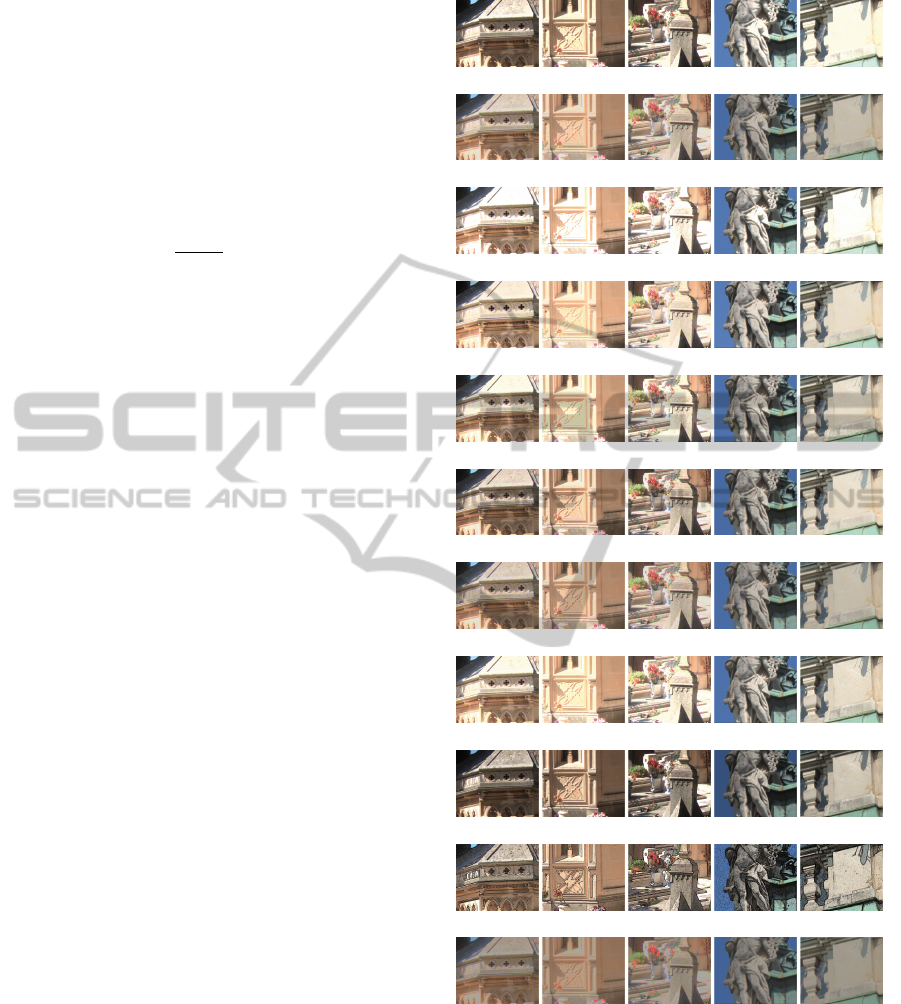
There are 27 single-shot HDR images in our eval-
uation set featuring a broad range of scenes with
higher and lower overall contrast and more or less
scenic details. Due to space constraints we present
only cropped results from two different scenes in fig-
ure 6 obtained for every algorithm.
(a) Linear with 5% cut-off
(b) Global photographic without burning
(c) Global photographic with burning
(d) Dynamic scene key
(e) Local photographic
(f) Local photographic with modified normalization
(g) Region-based global photographic without burning
(h) Region-based with adaptive unsharp masking
(i) Region-based with linear mapping
(j) Comic algorithm
(k) Adaptive logarithmic (by Drago)
Figure 6: Cropped images from LDR results of various tone
mapping algorithms as described in this paper.
4.1 Quantitative Evaluation
For the quantitative evaluation we chose the follow-
ing criteria: correlation ratio, signal-to-noise ratio,
global contrast, and local contrast. The correlation
ratio measures the correlation between an LDR im-
VISAPP2014-InternationalConferenceonComputerVisionTheoryandApplications
150
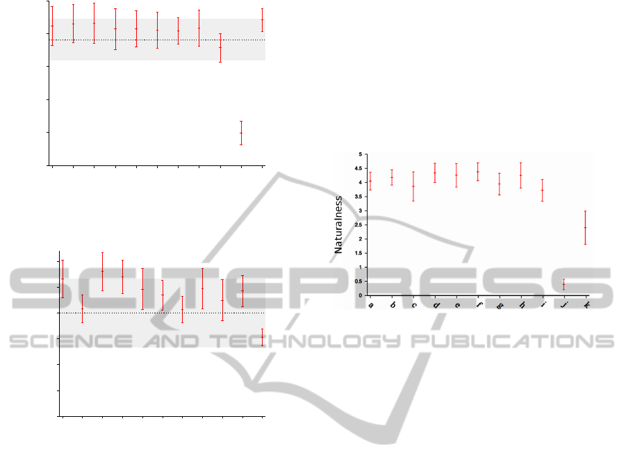
20
25
30
35
40
45
a
b
c
d
e
f
g
h
i
j
k
SNR
Figure 7: Average SNR values and standard deviations of
LDR images. The shaded area denotes the SNR and stan-
dard deviation of the original HDR images for comparison.
0
0.05
0.1
0.15
0.2
0.25
0.3
a
b
c
d
e
f
g
h
i
j
k
RMS (G)
Figure 8: Average RMS contrast and standard deviations of
LDR images. The shaded area denotes the RMS and stan-
dard deviation of the original HDR images for comparison.
age and its original HDR scene by using the Pearson
coefficient. Global and local contrast were both mea-
sured using the RMS contrast approach (Frazor and
Geisler, 2006), whereby the global contrast was mea-
sured for the whole image and the local contrast result
is the average of multiple windowed RMS measure-
ments. Results of the SNR and global contrast mea-
sures are depicted in figures 7 and 8 (please refer to
figure 6 for identifying the different algorithms). It
can be noted that the results greatly differ from each
other, but that there is no clear winner, so trade-offs
have to be made. In the figures, however, we have
also indicated the variance of those quantitative mea-
sures within the original image set of 12bit data. We
have experienced that a good tone mapping algorithm
should have values whose mean lies well within this
shaded stripe, and whose top values perform little bet-
ter than on the original data although their range of
variance should preferably be small.
4.2 Qualitative Evaluation
We chose a small control group of five students who
are experienced in image processing. Every tone
mapped LDR image was rated with values between 0
for poor and 5 for exceptional performance within the
following qualitative categories: brightness, global
contrast, local contrast, textural details, artifacts, fi-
delity, and naturalness. It is however very diffi-
cult to distinguish between some of these categories
because participants sometimes have different ideas
about those concepts like contrast vs. textural details.
Figure 9: Average subjective naturalness and standard devi-
ations of LDR images.
We exemplarily show the results for the subjec-
tively perceived naturalness in figure 9. To summarize
all subjective results we compiled a table of the final
ranks. We chose to create composite measures where
we evaluate the naturalness with respect to other de-
sired image features like contrast (global and local)
and textural detail. From table 1 it can be concluded
that algorithms f and d (compare with figure 6) show
good overall perceptual performance. It is interesting
to note that algorithm f did not modify the original al-
gorithm e but only the tonal normalization: as can be
seen from the table, this had a great effect on its rank.
Algorithm d is based on b with the intend to enhance
the global contrast which greatly succeeded. At the
same time the detail reproduction of d is worse then
that of b which is a direct consequence of increasing
global contrast (Smith et al., 2006), and the evaluation
data exactly reflects that.
4.3 Discussion
According to figure 9 algorithms d, e and f perform
best on average concerning the perceived naturalness,
whereby d and f also show a reasonably small vari-
ance over the whole set of images. These two algo-
rithms are also ranked best in our comparison table 1
whereby d creates higher perceived contrast but f is
better balanced between image contrast and preserv-
ing textural detail. These characteristics are verified
by our quantitative measurements where d is second
best in terms of RMS contrast as shown in figure 8 and
ToneMappingforSingle-shotHDRImaging
151

Table 1: Rank of the subjective visual performance.
C = Contrast, D = Details, N = Naturalness
Rank C D C/N D/N C/D/N
1 d k d f f
2 j f f b d
3 c g h e h
4 h b e h e
5 i e a d b
6 a h c g g
7 e d i a a
8 f a b i i
9 g i g c c
10 b c j k k
11 k j k j j
f is clearly worse but still within the upper range con-
cerning the original 12bit RMS values. Therefore, we
can recommend algorithm d as a tone mapper in in-
dustrial image processing applications where fast ac-
quisition times and high-contrast images are needed.
5 CONCLUSIONS
We have presented a unified framework and modi-
fied tone mapping operators for the purpose of single-
shot HDR imaging. The goal was to enhance the vi-
sually perceived contrast of tone mapped LDR im-
ages, thereby preserving most textural detail of the
original HDR images in both bright and shadowed
regions. The qualitative evaluation shows that this
was successfully achieved with our newly introduced
dynamic scene key approach. It has been shown
that the implementation of tonal normalization after
tonal compression should be taken care of because
the clamping strategy for out of range intensities has
a measurable effect on the subjective perception of
the mapping result. Finally, we introduced a region-
based noise reduction and selective sharpening ap-
proach that can be added to the general tone mapping
framework in order to enhance the performance of al-
ready existing mapping operators. In our evaluation
section we have outlined general criteria for subjec-
tive evaluation of tone mapping results.
REFERENCES
Bodrogi, P. and Khanh, T. Q. (2012). Illumination, Color
and Imaging: Evaluation and Optimization of Visual
Displays. Wiley Series in Display Technology. Wiley-
VCH Verlag GmbH & Co. KGaA.
DiCarlo, J. M. and Wandell, B. A. (2000). Rendering high
dynamic range images. Sensors and Camera Systems
for Scientific, Industrial, and Digital Photography Ap-
plications, 3965:392–401.
Drago, F., Myszkowski, K., Annen, T., and Chiba, N.
(2003). Adaptive logarithmic mapping for displaying
high contrast scenes. In Brunet, P. and Fellner, D. W.,
editors, Proc. of EUROGRAPHICS, Computer Graph-
ics Forum, pages 419–426. Blackwell Pub.
Felzenszwalb, P. F. and Huttenlocher, D. P. (2004). Effi-
cient graph-based image segmentation. International
Journal of Computer Vision, 59:167–181.
Frazor, R. A. and Geisler, W. S. (2006). Local lumi-
nance and contrast in natural images. Vision Research,
46:1585–1598.
Immerkær, J. (1996). Fast noise variance estimation. Com-
puter Vision and Image Understanding, 64:300–302.
Kuhna, M., Nuutinen, M., and Oittinen, P. (2011). Method
for evaluating tone mapping operators for natural high
dynamic range images. In Imai, F. H. and Xiao, F.,
editors, Digital Photography VII, SPIE Proc., pages
78760O–78760O–12. SPIE.
Ledda, P., Chalmers, A., Troscianko, T., and Seetzen, H.
(2005). Evaluation of tone mapping operators using
a high dynamic range display. ACM Transactions on
Graphics, 24:640–648.
Mantiuk, R., Tomaszewska, A., and Heidrich, W. (2009).
Color correction for tone mapping. In Dutr, P. and
Stamminger, M., editors, Proc. of EUROGRAPHICS,
Computer Graphics Forum, pages 193–202. Black-
well Pub.
Reinhard, E. (2002). Parameter estimation for photographic
tone reproduction. J. of Graphics Tools, 7:45–52.
Reinhard, E., Heidrich, W., Debevec, P., Pattanaik, S.,
Ward, G., and Myszkowski, K. (2010). High Dynamic
Range Imaging: Acquisition, Display, and Image-
Based Lighting. Morgan Kaufmann, 2nd edition.
Reinhard, E., Stark, M., Shirley, P., and Ferwerda, J. (2002).
Photographic tone reproduction for digital images.
ACM Transactions on Graphics, 21:267–276.
Smith, K., Krawczyk, G., Myszkowski, K., and Seidel, H.-
P. (2006). Beyond tone mapping: Enhanced depiction
of tone mapped HDR images. Computer Graphics Fo-
rum, 25:427–438.
VISAPP2014-InternationalConferenceonComputerVisionTheoryandApplications
152
