
Activity Recognition Using Non-intrusive Appliance Load Monitoring
Olaf Wilken, Oliver Kramer, Enno-Edzard Steen and Andreas Hein
University of Oldenburg, Oldenburg, Germany
Keywords:
Activity Recognition, Non-intruisve Appliance Load Monitoring.
Abstract:
The recognition of sequences via non-intrusive appliance load monitoring has an important part to play for
various applications in healthcare. In our work, we present a system for the detection of daily activities based
on the use of appliances. The objective of our activity monitoring system is to maximize the time elder people
can stay in their own domestic environment. We propose a system that is able to detect comparably complex
activities that may be interrupted by other activities. In the experimental part of our work, a one-month and a
half-year field study demonstrate the capabilities of the proposed approach.
1 INTRODUCTION
In the context of the demographic change, new tech-
nologies become more and more important to pre-
serve the independence of elder people. Here, the
focus lies on the recognition of activities of daily liv-
ing (ADL, e.g. toileting) (Katz et al., 1963) and in-
strumental activities of daily living (IADL, e.g. cook-
ing) (Katz, 1983) and the detection of deviations from
these usual activities. When deviations are detected,
the alert states can be used to inform assistants like
relatives or nurses. The main objective of such a sys-
tem is to let elder people live in their domestic envi-
ronments independently as long as possible.
Various approaches for activity recognition with dif-
ferent types of sensors are known in literature: body-
worn sensors as RFID reader (Philipose et al., 2004),
ambient intrusive sensors as vision sensors (Nguyen
et al., 2005; Oliver et al., 2002) or microphones (Chen
et al., 2005) or ambient non-intruisve sensors as mo-
tion sensors (Virone et al., 2008; Barger et al., 2005;
Guralnik and Haigh, 2002), state sensors (Kasteren
et al., 2008) or power sensors (Noury et al., 2011).
The classification of the sensor types in the above cat-
egories is given in (Ni Scanaill et al., 2006). Fur-
thermore all systems, which are not based on vision
sensors are called sensor-based activity recognition
systems. A detailed overview of sensor-based ac-
tivity recognition systems is given in (Chen et al.,
2012). An overview of vision-based systems is given
in (Poppe, 2010; Moeslund et al., 2006). Most ac-
tivity recognition systems try to infer predefined ac-
tivities with the help of probabilities. Therefore, un-
known individual activities can be filtered out by pre-
defined activities. This can lead to a loss of infor-
mation. Furthermore, a lot of systems were evalu-
ated by simplified scenarios with single activities, but
in the real world the activities are complex (paral-
lel/interrupting activities) (Chen et al., 2012). The
system we propose in this work detects daily indi-
vidual activities without inference of any predefined
activities and the evaluation was executed in two field
studies. The activity recognition based on power sen-
sors installed in a fuse box that first classifies ap-
pliances by decomposition of total load. These sys-
tems are called non-intrusive appliance load moni-
toring (NIALM) cf. (Hart, 1992). Our algorithm is
able to detect possible activities without specified pre-
settings. In most cases, the labels of detected activi-
ties can be inferred with the help of the associated ap-
pliances. Furthermore, the developed system is able
to handle noisy data, e.g., wrong classified appliances
or little variations in the sequences of the same activ-
ities, and is able to detect complex activities, which
can be interrupted by other activities and can also
recognize parallel/interrupting activities. The main
components of the system are NIALM and activity
recognition. In contrast to the system we propose in
this work, the approach by Noury etal (Noury et al.,
2011) requires the manual specification of activities
with the association of appliances for each installa-
tion and one sensor for each appliance to be classi-
fied is used (called intrusive appliance load monitor-
ing (IALM) cf. (Hart, 1992)).
This work is structured as follows. The NIALM pro-
cedure of our system is introduced in Section 2 de-
40
Wilken O., Kramer O., Steen E. and Hein A..
Activity Recognition Using Non-intrusive Appliance Load Monitoring.
DOI: 10.5220/0004700300400048
In Proceedings of the 4th International Conference on Pervasive and Embedded Computing and Communication Systems (PECCS-2014), pages 40-48
ISBN: 978-989-758-000-0
Copyright
c
2014 SCITEPRESS (Science and Technology Publications, Lda.)
scribing the sensors, the edge detection and the appli-
ance recognition procedure. Section 3 describes our
approach to detect activities as sequences of switch-
ing events. In Section 4, the behavior of our system is
shown in two field studies. The article closes with a
summary of the most important results in Section 5.
2 NON-INTRUSIVE APPLIANCE
LOAD MONITORING
2.1 Sensor
From the employed power sensor (CRD5110 from
CR Magnetics (Magnetics, 2013)), the electrical pa-
rameters voltage (V
RMS
), current (I
RMS
) and real
power (P) are streamed with a sampling rate of 5 Hz.
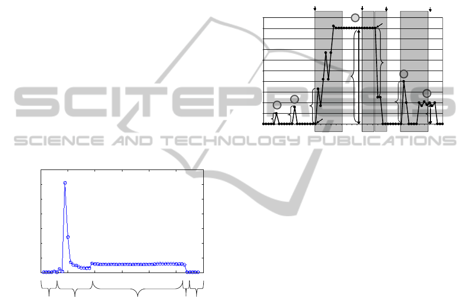
In Figure 1, the typical signal of an active appliance
is shown. The signal has a transitive noise (transient)
at the turn-on phase. Afterwards, a plateau (steady
state) follows with only small variations in contrast to
the transient. The turn-off phase is only an edge.
0 10 20 30 40 50 60
0
200
400
600
800
1000
1200
1400
Datenpunkte
Wirkleistung [W]
steady
transient edge
data points
steady
steady
real power [W]
Figure 1: A signal of a running appliance from power sen-
sor.
2.2 Edge Detection
The edge detection module recognizes switchings of
appliances with real power P(k) above a threshold θ
2
in the steady state. This threshold separates events
generated by appliances from noise. In order to deter-
mine the real power in the steady state, two different
thresholds θ
1
and θ
2
and two time slots of different
lengths (σ
1
and σ
2
) are employed. The first thresh-
old θ
1
determines the beginning of a possible switch-
ing. For the determination of θ
2
, two time slots are
used, one for the turn-on phase and the other for the
turn-off phase. The turn-on time slot is longer, be-
cause the corresponding transient noise takes longer
time. For example, the noises (signal one, two and
five) in Figure 2 are filtered out, and the correct
switches from the third signal will be detected by this
procedure. The detection of turn-on and turn-off is
computed with equation 1, where “1” represents turn-
on and “-1” represents turn-off. For a robust detec-
tion of turn-offs, two time slots with the same size are
used. In order to eliminate noise in the stable state,
the median is computed over a short period of one
second.
0
10
20
30
40
50
60
70
80
90
100
0 2 4 6 8 10 12 14 16 18 20 22 24 26 28 30 32 34 36 38 40 42 44 46 48 50 52 54 56 58 60 62 64 66 68
Datenpunkte
Wirkleistung [ W ]
Θ
1
>
1
2
3
4
5
turn on
turn off
Θ
2
<
Θ
2
>
Θ
1
<
>Θ
1
Θ
1
>
Θ
1
<
real power [W]
data points
t+σ
1
t- σ
2
t+ σ
2
t+ σ
1
Figure 2: Example data for edge detection from turn-on/off
event of an appliance (θ
1
= 25 W , θ
2
= 45 W ,σ
1
= 10 data-
points, σ
2
= 5 datapoints, ). The length of the turn-on phase
is σ
1
and the length of turn-off is σ
2
, respectively.
f (k) =
1 P(k + 1) − P(k) ≥ θ
1
∧
P(k + σ
1
) − P(k) ≥ θ
2
−1 P(k + 1) − P(k) ≤ −θ
1
∧
P(k − σ
2
) − P(k + σ
2
) ≥ θ
2
0 else (no switch)
(1)
For each data point step with a switch event, the de-
vice recognition module is run.
2.3 Feature Extraction
The device classification is described in the following.
The question arises, which features are appropriate
for the device recognition task. The streamed elec-
trical parameter voltage V
RMS
is not stable enough:
if appliances are running in parallel, the voltage
varies (voltages variations have also been detected by
Hart (Hart, 1992)). After each switching of an appli-
ance, the voltage changes a little bit. This has neg-
ative implications for the recognition of the second
appliance. As the power P(k) depends on the voltage,
P(k) = V
RMS
(k) · I
RMS
(k) · cosα (2)
with phase shift α, it is no appropriate stable fea-
ture. In contrast, the voltage-independent effective
resistance R(k) is a suitable feature for the appliance
ActivityRecognitionUsingNon-intrusiveApplianceLoadMonitoring
41

recognition problem. It can simply be computed from
the sensor data with
R(k) =
V
RMS
(k)
I
RMS
(k) · cosα
=
V
2
RMS
(k)
P(k)
. (3)
This equation is also employed for the values of
the turn-on/turn-off signal from a running appliance.
However, if two or more appliances are running si-
multaneously, the computation of effective resistance
values R
A
has to consider that the appliances are con-
nected in parallel. Therefore, the following equation
has to be applied:
R
A
(k) =
1
1
R(k)
−
1
R(k
0
−2)
;k ∈ [k
0
+ 2, k
0
+ n] (4)
R
A
(k) =
1
1
R(k)
−
1
R(k
1
+2)
;k ∈ [k
1
, k
1
− n] (5)
with data point k
0
for the beginning of turn-on, data
point k
1
for the beginning of turn-off and n ∈ N
0
. In
order to distinguish appliances with similar effective
resistance (and similar real power), the resistance val-
ues after the turn-on are not sufficient. Since the sen-
sor (cf. Figure 1) provides a transient signal when
an appliance is turned on, it can be used for a bet-
ter distinction. During the analysis of the transient
signals from our appliances, we observed that the
first two measurements after different turn-ons of the
same appliance can be disturbed and vary too much.
Therefore, they are unsuitable for a robust recognition
and left out in the classification process. Mean value
and standard deviation of the turn-on phase are em-
ployed for classification of similar appliances. Turn-
off events do not have transient signals. The median
of the last measured values before turn-off is used
in combination with the information, which device is
running, i.e., the turn-on information. In contrast to
feature extraction real power for edge detection is suf-
ficient because the impact of variations is here not so
important.
For the classification process, K-nearest-
neighbors (Cover and Hart, 1967), na
¨
ıve
Bayes (Mitchell, 1997) and decision
trees (C4.5) (Quinlan, 1993) have been used. A
comparison of the employed classifiers will be shown
in the experimental section.
3 ACTIVITY RECOGNITION
The activity recognition is based on sequence recog-
nition. A sequence is an order of letters which repre-
sent classified appliance switchings. Each appliance
switching AS
i
is coded by a letter in the sequence. An
uppercase letter represents a turn-on event, and the
corresponding lowercase represents a turn-off. For
example, the coded letters for the event “toaster on” is
T and for the event “toaster off” is t. The information
that an appliance switching pair (turn-on/turn-off) can
directly be mapped to an activity is considered as sim-
ple and robust case (e.g. turn-on/turn-off of “TV” are
associated to activity “watching television”). Activi-
ties can be divided into two types:
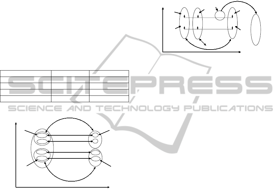
1. A simple activity is represented by an interlaced
sequence containing complete pairs of appliance
turn-on and corresponding turn-off events that be-
long together. For example, in Figure 3 S
2
is a
simple activity (closed sequence).
2. A complex activity contains at least two non-
closed sequences, with a begin sequence and an
end sequence. The begin sequence contains at
least one turn-on event, but no corresponding
turn-off. The end sequence contains all missing
turn-off events. Figure 3 shows an example. Se-
quence S
1
is a begin sequence, S
3
is a intermediate
sequence, and S
4
is an end sequence of a complex
activity. S
2
is a parallel/interrupting activity.
The steps of the activity recognition process are de-
scribed in the following.
3.1 Detection of Sequences
Our observations show that a sequence with a large
number of switching events corresponds to an activ-
ity. Hence, switching events that occur in quick suc-
cession potentially belong to the same sequence. A
switching event AS
j
is assigned to a sequence S
i
em-
ploying the following criterion:
{AS
j
∈ S
i
| time(AS
j
)−time(AS
j−1
) < T ∧AS
j−1
∈ S
i
}
(6)
with threshold T being the maximum time between
two switchings that belong to the same sequence. Af-
ter this time-based clustering, each sequence is clas-
sified as closed or not. Again, Figure 3 illustrates the
creation of sequences.
3.2 Detection of Related Sequences
In this section, the begin sequences BS
i
, the end se-
quence ES
i
and intermediate sequences IS
i
of the
complex activity candidates CAC
i
are determined.
The result of the created structure from the complex
activity candidates is
CAC
i
=
BS
j
i
| BS
j
∈ {S
1
, . . . , S
n
}
ES
k
i
| ES
k
∈ {S
1
, . . . , S
n
}
{IS
p
i
, . . . , IS
s
i
} | {IS
p
, . . . , IS
s
} ⊂ {S
1
, . . . , S
n
}.
(7)
PECCS2014-InternationalConferenceonPervasiveandEmbeddedComputingandCommunicationSystems
42

F D A T t
S
1
d
S
2
S
3
M O o m
time
S
4
time
f a
F D A T t
M O o m
d
f a
closed
not
closed
not
closed
not
closed
Figure 3: Example data for creation of sequences. F = “ceil-
ing light (living room)” on; D = “TV (living room)” on; A
= “table lamp (living room)” on; T = “standard lamp (liv-
ing room)” on; M = “ceiling light (floor)” on; O = “ceil-
ing light (bathroom)” on. The lowercase letters represent
turn-off events. Sequences S
1
, S
3
and S
4
represent the com-
plex activity “watching TV & reading” and S
2
represents
the simple activity “toileting”.
Every closed sequence is a candidate for a simple ac-
tivity EAC
i
. In Figure 4, an example of two complex
activity candidates CAC
1
, CAC
2
and one simple activ-
ity candidate EAC
1
is shown. In this example the de-
teremined candidates are the ground truth, but it may
occur in real situations that the complex activity may
contain the two complex activity candidates CAC
1
,
CAC
2
(transitive dependency), and the sequence S
2
can be an intermediate sequence of a complex activ-
ity. These dependencies are solved in the following
steps.
time
CAC
1
F D A T t
S
1
S
2
M O o m
S
5
f a
K
S
4
CAC
2
k
S
6
BS
1
ES
1
BS
2
ES
2
IS
1
IS
1
IS
2
1
2
4
4
5
5
6
EAC
1
d
S
3
IS
1
3
Figure 4: Example data for detected start sequences, inter-
mediate sequences and end sequences of two complex ac-
tivity candidates. The letters represent the same appliance
switchings as in Figure 3 with additonal K = “desk lamp”
on and complex activity “desk work” consisting of S
4
and
S
6
.
3.3 Clustering of Sequences
In this section, all sequences are clustered based on
the feature similarity considering variations of the
same sequences. For example, the variations can be
wrong classified appliances, permutations of switch-
ings or missing events. For the detection of such vari-
ations, the distance of two sequences is computed by
an extended edit distance (Oommen, 1997). The edit
distance is defined as the transformation from one se-
quence to another sequence with a minimum number
of operations (Levenshtein, 1966). The operations are
deletion, insertion, and replacement. With the ex-
tended edit distance the additional operation transpo-
sitions allows the detection of adjacent transpositions.
Furthermore, the extended edit distance supports sub-
stitution matrices to recognize wrong classified appli-
ances, and the weights of all operations can be chosen
freely. It is computed employing dynamic program-
ming techniques. The two sequences S
1
and S
2
, which
have to be compared, constitute columns and rows of
a matrix D defined as
D
i, j
= min
D
i−1, j
+W
d
(deletion)
D
i, j−1
+W
i
(insertion)
D
i−1, j−1
+ s(S
1
(i), S
2
( j)) S
1
(i) 6= S
2
( j)
D
i−1, j−1
S
1
(i) = S
2
( j)
D
i−2, j−2
S
1
(i) = S
2
( j − 1)
∧
S
1
(i − 1) = S
2
( j)
(8)
with n = |S
1
| and m = |S
2
|. Function s(·) computes
the weights of replacements (e.g. from the substitu-
tion matrix), and W
d
,W
i
are weights of the operations
deletion and insertion. The matrix is initialized with
D
0,0
= 0, D
i,0
= i, 1 ≤ i ≤ m and D
0, j
= j, 1 ≤ j ≤ n.
The entry D
m,n
defines the distance computation.
The agglomerative hierarchical clustering method is
used for the clustering process. The distance measure
that we employ computes the relation of similarity be-
tween two sequences with the help of the extended
edit distance
δ = 1 −
D
m,n
max(| S
1
|, | S
2
|) ∗ max(W
d
,W
i
,W
s
)
(9)
with weights W
s
of replacement. The results of the
clustering step are similarity activity clusters ACl
i
=
{S
j
. . . S
n
}. For example when complex activity from
Figure 3 appears on different days then all three dif-
ferent sequences are in three different clusters.
3.4 Detection of Activity Candidate
Clusters
Not all sequences in a similarity activity cluster ACl
i
have to be associated with the same activity. For ex-
ample, a start sequence of a complex activity candi-
date CAC
1
may be an element of ACl
i
, and the associ-
ated end sequence may be element of ACl
j
. Another
start sequence of CAC
3
may also be element of ACl
i
,
but the associated end sequence is element of ACl
k
.
Hence, the two complex activity candidates are as-
sociated with different activities (cf. Figure 5). The
correct association activity is solved by computing ac-
tivity candidate cluster CAC
Cl
i
with
| {CAC
i
| BS
m
i
∈ ACl
j
, ES
q
i
∈ ACl
l
} |≥ H. (10)
ActivityRecognitionUsingNon-intrusiveApplianceLoadMonitoring
43
The threshold H is the minimum number of occur-
rence of a daily activity. Furthermore, it can happen
that a similar activity cluster ACl
i
may contain either
closed sequences that are associated to a simple ac-
tivity candidate or contain non-closed sequences that
can be associated with a complex activity candidate.
These clusters are simple activity candidate clusters
EAC
Cl
i
, if all closed sequences exceed the threshold
S
E
and all sequences, except the sequences which are
associated to a complex activity candidate, on differ-
ent days are larger than threshold H. The result of the
correct solved association is shown in Table 1. In the
next step, intermediate sequences of complex activity
candidate clusters are determined.
Table 1: Assignments of similarity cluster and activity can-
didates.
Activity candidate cluster Similitary activity Activity candidate
CAC
Cl
p
ACl
i
, ACl
j
{CAC
k
, . . . ,CAC
m
}
CAC
Cl
q
ACl
i
, ACl
r
{CAC
f
, . . . ,CAC
n
}
. . . . . . . . .
EAC
Cl
t
ACl
j
{EAC
w
, . . . , EAC
z
}
F D T t
ACl
i
F D T t
F D T t
ACl
j
f d
ACl
k
f d
K d f k
K d f k
F D T t
{ACl
i
,ACl
k
}
{ACl
i
,ACl
j
}
CAC
1
CAC
2
CAC
3
CAC
4
BS
1
BS
4
ES
1
ES
4
p
q
t
s
days
time
Figure 5: Example data for correct association of similarity
activity clusters (CAC
1
,. . . ,CAC
4
) with two different com-
plex activity candidate clusters. The letters represent the
same appliance swichtings as in Figure 4. CAC
1
and CAC
2
are associated to activity (candidate cluster) “watching TV
at night” and CAC
3
and CAC
4
are associated to “watching
TV & desk work at afternoon”.
3.5 Detection of Activities
In the last step, the intermediate sequences, which can
also be activity candidate clusters, are determined.
All the activity candidate clusters, which either are
not associated to another activity candidate cluster or
in which all the dependencies, the intermediate se-
quences, are solved, are the result activities A
i
(simple
activities EA
i
or complex activities CA
i
). First, every
intermediate sequence of CAC
i
∈ CAC
Cl
j
is examined,
if it is element of all other CAC
n
∈ CAC
Cl
j
. Figure 6
shows the sequence d ∈ ACl
t
that is associated to all
CAC
n
. The number of elements in ACl
t
is equal (or
approximately equal) to elements of CAC
Cl
j
, there-
fore, ACl
t
with its elements is associated to CAC
Cl
j
.
However, the sequence Kk ∈ ACl is not associated to
CAC
Cl
j
, because this one occurs only once. Second,
F D
ACl
j
F D
CAC
i
BS
i
BS
n
ES
i
ES
n
:
CAC
n
f
ACl
m
f
:
d
ACl
t
d
:
:
K k
IS
i
K k
ACl
z
K k
:
IS
i
p
q
l
s
r
v
CAC
j
Cl
days
time
Figure 6: Example data for association of intermediate
sequences to complex activity candidate cluster CAC
Cl
j
.
The letters represent the same appliance switchings as in
Figure 4. Here the sequence “Kk” (representing activ-
ity “desk work”) is a parallel/interrupting activity in CAC
i
.
CAC
i
,. . . ,CAC
n
represent the complex activity “watching
TV”.
the transitive dependencies are recursively solved, but
this never ocurred in our executed studies. Further-
more, an element of detected activities is parallel or
interrupting, if it sometimes occurs in another activ-
ity. For example, in Figure 6, the sequence Kk can be
a parallel/interrupting activity.
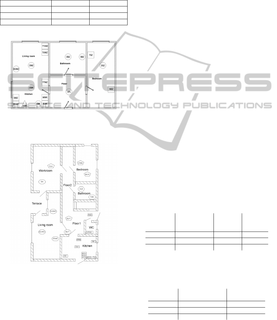
4 EVALUATION
For the experimental evaluation of the system, we
conducted two field studies. The first study was car-
ried out in a two-room apartment (cf. Figure 7), the
second study in a three-room apartment (cf. Figure 8).
In every apartment, an elderly person over 70 years
old lived alone during the study. For every electric
circuit, a power sensor was installed in the fuse box.
Eighteen appliances in the two-room apartment and
twenty-two appliances in the three-room apartment
were monitored (cf. Table 2). Appliances under the
threshold of P = 35 W have not been monitored (i.e.,
a radio and two energy saving bulbs in the first study,
and eight energy saving bulbs in the second study).
During the installation of the system, each appliance
was learned by two or three training data in a su-
pervised way. Every resident was asked to log the
switchings of appliances and the corresponding ac-
tivities (e.g. “meal preparation”). Since the logs are
usually incomplete (Kasteren et al., 2008), a wireless
motion sensor was installed in every room for further
manual labeling of appliance switchings. In the first
study, 28 days and in the second study, 18 days of
PECCS2014-InternationalConferenceonPervasiveandEmbeddedComputingandCommunicationSystems
44
activities have manually been labeled. For the activi-
ties ground truth does not exist, because the logs were
incomplete and the activities could not manually be
labeled in contrast to switching appliances.
Table 2: Overview of the installations used in the field stud-
ies.
Apartments 2-room apartment 3-room apartment
No. of electric circuit 3 4
No. of appliances 18 22
Period of data collection 5 months 1 month
Figure 7: Floor plan of 2-room apartment. The acronyms
represent appliances and the shapes (e.g. circle) the associ-
ated electric circuits.
Figure 8: Floor plan of 3-room apartment. The acronyms
represent appliances and the shapes the associated electric
circuits.
4.1 Appliance Classification
In both field studies, the same thresholds (θ
1
= 35 W,
θ
2
= 20 W with window sizes σ
1
= 3 s (turn-on) and
σ
2
= 1 s (turn-off)) are used for edge detection. The
thresholds have been determined empirically in dif-
ferent tests. In the first study, 40 appliance switch-
ings of 2, 661 manually labeled switchings were not
detected correctly. In the second study, the detection
of seven switchings of 1, 518 manually labeled have
failed. The reason for the larger number of failures
in the first study was that two different light switches
were installed closely together. The test person could
execute two switchings of different appliances within
three seconds. But the edge detection can only detect
one switching within three seconds (due to the win-
dow size). The high number of appliance switchings
in first study was related to a defect refrigerator. This
one was active (turn-on/turn-off) every hour.
First, we compare the three classifiers K-nearest-
neighbors with K = 1 (1-NN) (Cover and Hart,
1967), na
¨
ıve bayes (Mitchell, 1997) and decision
trees (C4.5) (Quinlan, 1993). For the classifier C4.5
Weka framework was used and the other both classi-
fiers have been implemented. Tables 3 and 4 show the
recognition accuracies w.r.t. different training sets.
In the first column of both tables, only the training
patterns generated during installation are used. For
the test data, all manually labeled patterns are used.
Here, the 1-NN classifier shows the best results with
over 96% accuracy. With an increase of the training
set size (second and third column), the precision of
1-NN only increases slightly in contrast to the other
classifiers. But in both studies, 1-NN achieves the
best results for each training set size. Since the gen-
eration of labeled training data during installation is a
realistic scenario, we emphasize that these results are
relevant in practice.
Table 3: Classification accuracy of the three classifiers w.r.t.
different training sets in the first experimental study (train-
ing data/test data). Training data from installation does not
contain the not detected edges (40 switchings).
2 - 3 training data
per appliance
(92/2621)
data of 1
week
(801/1912)
data of 2
weeks
(1454/1259)
1-NN 96.9% 97.9% 97.9%
C4.5 80.6% 96.6% 97.2%
na
¨
ıve bayes 91% 93.9% 94.2%
Table 4: Classification accuracy of the three classifiers
w.r.t. different training sets in the second experimental
study (training data/test data). Training data from installa-
tion does not contain the not detected edges (7 switchings).
2 - 3 training data per
appliance (122/1511)
data of 1 week
(816/817)
1-NN 96.2% 96.36%
C4.5 78.1% 95.96%
na
¨
ıve bayes 91.4% 94.14%
ActivityRecognitionUsingNon-intrusiveApplianceLoadMonitoring
45
With the extension that the turn-off events are clas-
sified depending on known turn-on events, the pre-
cision of the 1-NN classifier based on the installa-
tion training set is increased. The precision in the
first field study becomes 97.62%, the corresponding
value in the second study achieves 96.4%. Sensi-
tivity, specificity, positive predictive value (ppv) and
negative prediction value (npv) have been determined
for measure of performance fom 1-NN classifier with
extension. Specificity and negative prediction value
were between 97% and 100% for all appliances in
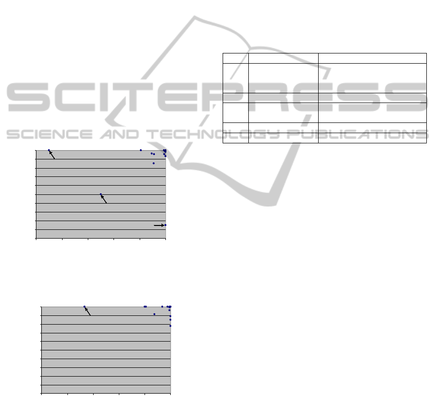
both studies. In the first study, there are three ma-
jor outliers in the sensitivity and positive predictive
value (cf. Figure 9). Appliance “table lamp” was
often wrongly classified as “shelf lighting” and vice
versa. The reason for this was that the two appliances
were very similar and the turn-on of “table lamp” was
often interrupted by noise of appliance “TV”. Further-
more, appliance “extracted hood” from first and sec-
ond study (cf. Figure 10) are rarely used (three in first
study and five times in second study). This appliance
was often wrong classified.
0%
10%
20%
30%
40%
50%
60%
70%
80%
90%
100%
0% 20% 40% 60% 80% 100%
positive predictive value (ppv)
sensitivity
shelf lighting
extraction hood
table lamp
Figure 9: Sensitivities and positive predictive value of all
appliances from first study.
0%
10%
20%
30%
40%
50%
60%
70%
80%
90%
100%
0% 20% 40% 60% 80% 100%
positive predictive value (ppv)
sensitivity
extraction hood
Figure 10: Sensitivities and positive predictive value of all
appliances from second study.
4.2 Activity Recognition
The activity recognition procedure is evaluated with
the complete data from both studies. The first study
contains data collect on 140 days (about five months),
the second study contains data from 27 days. The
number of different days with a daily activity (thresh-
old H of the activity recognition procedure) has been
determined empirically. This threshold was set to 100
days of 140 days in the first study and 17 days of 27
days in the second study, respectively. The two appli-
ances “table lamp in living room” and “shelf lighting
in living room” (cf. Figure 9) are often mixed up by
the appliance recognition (probability from the confu-
sion matrix). This was considered in the substitutions
matrix, cf. Equation 8.
Table 5: Simple activities of the first study (b = bathroom; f
= floor).
No. inferred activities appliances
A
1
toileting during day ceiling light (f) on; mirror lamp (b)
on; mirror lamp (b) off; ceiling
light (f) off
A
2
toileting during day mirror lamp (b) on/off
A
3
toileting during night bedside lamp on; mirror lamp (b)
on/off; bedside lamp off;
A
4
afternoon tea kettle on/off
A
5
various activities ceiling light (f) on/off
The threshold for the similarity of sequences (cf.
Equation 9) was set to 70% for both studies. The
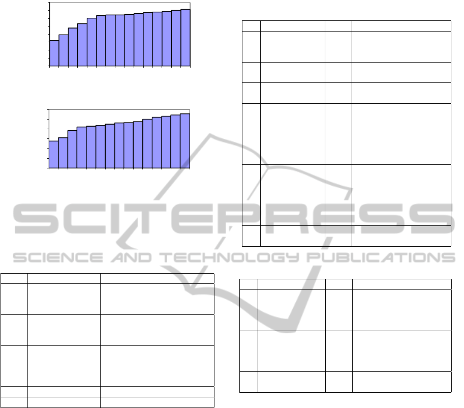
times for creating sequences (threshold T of Equa-
tion 6) was determined by histograms. The his-
tograms of both studies (cf. Figure 11) represent the
average number of appliances in sequence by time.
The average number of appliances was computed for
every time with the help of equation 6. For the thresh-
old T the times (bars from histograms) which show
the smallest distance of two adjacent bars have been
chosen (for first study T = 7 minutes and for second
study T = 8 minutes). Furthermore, stand-alone run-
ning appliances (e.g., the refrigerator) are filtered out
manually. Tables 5 and 6 show the detected simple
activities of both studies. In Tables 7 and 8 the de-
tected complex activities are shown with the associ-
ated similarity clusters ACl
i
. The tables also show
the positions (rooms) of some appliances for a clear
identification. The names of the activities are inferred
from the protocols and the involved appliances in the
tables. The order of the appliances in each activ-
ity is only one representative of several that have oc-
curred in reality. Some activities are recognized mul-
tiple times. For example, the simple activity “toilet-
ing during day” has been detected twice, because the
same activity is executed with different appliances.
The algorithms cannot distinguish between both ac-
tivities. Furthermore, two different activities can be
detected as one, e.g., the detected complex activity A
7
of the second study is in fact divided into the activities
“preparing morning coffee” and “preparing evening
PECCS2014-InternationalConferenceonPervasiveandEmbeddedComputingandCommunicationSystems
46
1,60
1,98
2,40
2,67
3,01
3,17
3,22
3,23
3,26
3,31
3,36
3,40
3,43
3,50
3,57
0,00
0,50
1,00
1,50
2,00
2,50
3,00
3,50
4,00
1 2 3 4 5 6 7 8 9 10 11 12 13 14 15
minutes
Mean number of applainces in
sequences
(a)
1,38
1,55
1,92
2,10
2,14
2,18
2,25
2,31
2,32
2,37
2,49
2,60
2,65
2,71
2,78
0,00
0,50
1,00
1,50
2,00
2,50
3,00
1 2 3 4 5 6 7 8 9 10 11 12 13 14 15
minutes
Mean number of appliances in
sequences
(b)
Figure 11: Histograms with an average number of appli-
ances in sequences at different times: (a) first study; (b)
second study.
Table 6: Simple activities of the second study (b = bath-
room; be = bedroom; f = floor).
No. inferred activities appliances
A
1
toileting during night ceiling light (be) on; ceiling light
(b) on; ceiling light (b) off; ceiling
light (be) off
A
2
toileting during day ceiling light (f) on; ceiling light (b)
on; ceiling light (b) off; ceiling
light (f) off
A
3
preparation for sleep ceiling light (f) on; ceiling light (b)
on; ceiling light (b) off; ceiling
light (be) on; ceiling light (f) off;
ceiling light (be) off
A
4
various activities ceiling light (be) on/off
A
5
various activities ceiling light (f) on/off
coffee”. For these activities, the same appliances are
used. This confusion can be solved by considering
the time of the day. It is possible that one similar-
ity cluster (ACl
i
) belongs to different activities, e.g.,
the detected complex activities A
9
and A
10
share the
same ACl
i
. If these two activities should be recog-
nized as one activity, the algorithm can be adapted
easily. Furthermore, only a few recognized activities,
which are named as various activities in the tables,
cannot be inferred to an unambiguous activity name,
because they appear in different activities. Finally,
there are sometimes larger variations (transpositions)
of elements in the same sequences, especially in long
sequences (e.g., A
3
in Table 6). The algorithm can
only detect adjacent transpositions. This issue is cur-
rently solved via the threshold H.
As parallel/interrupting activities, activity “toileting
during day” (A
1
of the first study) appeared in the ac-
Table 7: Complex activities of the first study (b = bathroom;
be = bedroom; f = floor; l = living room).
No. Inferred activities cluster appliances
A
6
breakfast ACl
1
ceiling light (l) on; kettle on;
kettle off
ACl
2
ceiling light (l) off
A
7
afternoon nap ACl
1
bedside lamp on
ACl
2
bedside lamp off
A
8
afternoon TV ACl
1
TV on
ACl
2
TV off
A
9
evening TV,
reading and
puzzles
ACl
1
ceiling light (l) on
ACl
2
TV on; table lamp (l) on
ACl
3
TV off; table lamp (l) off
ACl
4
ACl
1
of A
10
A
10
preparation for
sleep
ACl
1
mirror lamp (b) on; mirror
lamp (b) off; ceiling light (l)
off; ceiling light (be) on;
bedside lamp on; ceiling light
(be) off;
ACl
2
bedside lamp off
A
11
various activities ACl
1
ceiling light (f) on
ACl
2
ceiling light (f) off
Table 8: Complex activities of the second study (k =
kitchen).
No. Inferred activities cluster appliances
A
6
breakfast ACL
1
ceiling light (k) on; kettle on;
toaster on; kettle off; toaster
off
ACl
2
ceiling light (k) off
A
7
preparing morning
coffee/ evening
coffee
ACl
1
ceiling light (k) on; kettle
on/off
ACl
2
ceiling light (k) off
A
8
preparing meal ACl
1
hood light on
ACl
2
hood light off
tivities (A
8
and A
9
) with longer duration. In the sec-
ond study, no parallel/interrupting activities were de-
tected. This is certainly associated with the fact that
the detected complex activities had a shorter duration.
5 CONCLUSIONS
In our two experimental studies, we were able to
demonstrate the capabilities of our system for activ-
ity recognition based on appliance switchings. The
approach is capable of detecting simple and complex
activities. Furthermore, the algorithm can detect par-
allel/interrupting activities and can consider noise as
wrong classified appliances. A major problem eval-
uating the activity detection occured in verifying the
ground truth since the logs were incomplete. Further-
more, evening activities could not be recognized in
the second study since energy saving bulbs have been
ActivityRecognitionUsingNon-intrusiveApplianceLoadMonitoring
47

used. They can not be detected by the appliance de-
tection. An increased use of saving bulbs could lead
to future problems of activity recognition, because
the recognized activities of the two studies often in-
clude lamps. Furthermore, when at the beginning and
at the end of the day an appliance is switched (e.g.
“aquarium lighting”) the presented algorithm for ac-
tivity recognition would identify the various activities
during the day as one activity. This case did not oc-
cur in the two studies. One approach to solve this
could be a maximum time duration that a valid activ-
ity can have. Some recognized activities can be easily
determined by specifying significant appliances (e.g.
activity “breakfast” often contains appliance “toaster”
and “kettle”). But other activities that are not previ-
ously known or are very individual turn out to be dif-
ficult to detect (e.g. “afternoon nap”). The presented
approach is able to recognize such activities in an un-
supervised kind of way. In future works, we plan to
investigate, if the number of days with daily activi-
ties can be increased by recognizing larger transpo-
sitions of elements in sequences instead of only ad-
jacent transpositions. Furthermore, it will be inves-
tigated, how stand-alone running appliances, e.g., re-
frigerators, can be detected automatically.
REFERENCES
Barger, T. S., Brown, D. E., and Alwan, M. (2005). Health-
status monitoring through analysis of behavioral pat-
terns. Trans. Sys. Man Cyber. Part A, 35(1):22–27.
Chen, J., Zhang, J., Kam, A., and Shue, L. (2005). An auto-
matic acoustic bathroom monitoring system. In Inter-
national Symposium on Circuits and Systems (ISCAS
2005), pages 1750–1753 Vol. 2. IEEE.
Chen, L., Hoey, J., Nugent, C., Cook, D., and Yu, Z. (2012).
Sensor-based activity recognition. IEEE Transactions
on Systems, Man, and Cybernetics, Part C, 42(6):790
–808.
Cover, T. and Hart, P. (1967). Nearest neighbor pattern clas-
sification. IEEE Transactions on Information Theory,
13(1):21 –27.
Guralnik, V. and Haigh, K. Z. (2002). Learning mod-
els of human behaviour with sequential patterns. In
Proceedings of the AAAI-02 workshop Automation as
Caregiver, pages 24–30. AAAI Press.
Hart, G. (1992). Nonintrusive appliance load monitoring.
Proceedings of the IEEE, 80(12):1870–1891.
Kasteren, T. v., Noulas, A., Englebienne, G., and Kr
¨
ose, B.
(2008). Accurate activity recognition in a home set-
ting. In Proceedings of the 10th international confer-
ence on Ubiquitous computing, pages 1–9. ACM.
Katz, S. (1983). Assessing self-maintenance: activities of
daily living, mobility, and instrumental activities of
daily living. Journal of the American Geriatrics Soci-
ety, 31(12):721–727.
Katz, S., Moskowitz, R., Ba, J., and Jaffe, M. (1963). Stud-
ies of illness in the aged: The index of adl: a stan-
dardized measure of biological and psychosocial func-
tion. Journal of the American Medical Association,
185(12):914–919.
Levenshtein, V. I. (1966). Binary Codes Capable of Cor-
recting Deletions, Insertions and Reversals. Soviet
Physics Doklady, 10:707–710.
Magnetics (2013). CR Magnetics CRD5110.
http://www.crmagnetics.com/Products/CRD5100-
Series-P30.aspx. Accessed: 2013-07-28.
Mitchell, T. M. (1997). Machine Learning. McGraw-Hill,
Inc., New York, NY, USA, 1 edition.
Moeslund, T. B., Hilton, A., and Kr
¨
uger, V. (2006). A
survey of advances in vision-based human motion
capture and analysis. Comput. Vis. Image Underst.,
104(2):90–126.
Nguyen, N. T., Phung, D. Q., Venkatesh, S., and Bui, H.
(2005). Learning and detecting activities from move-
ment trajectories using the hierarchical hidden markov
models. In In Proceedings of IEEE International Con-
ference on Computer Vision and Pattern Recognition,
pages 955–960. IEEE Computer Society.
Ni Scanaill, C., Carew, S., Barralon, P., Noury, N., Lyons,
D., and Lyons, G. M. (2006). A review of approaches
to mobility telemonitoring of the elderly in their liv-
ing environment. Annals of Biomedical Engineering,
34(4):547–563.
Noury, N., Berenguer, M., Teyssier, H., Bouzid, M. J., and
Giordani, M. (2011). Building an index of activity of
inhabitants from their activity on the residential elec-
trical power line. IEEE Transactions on Information
Technology in Biomedicine, 15(5):758–766.
Oliver, N., Horvitz, E., and Garg, A. (2002). Layered rep-
resentations for human activity recognition. In Pro-
ceedings of the 4th IEEE International Conference on
Multimodal Interfaces, page 3. IEEE Computer Soci-
ety.
Oommen, B. J. (1997). Pattern recognition of strings
with substitutions, insertions, deletions and general-
ized transpositions. Pattern Recognition, 30(5):789–
800.
Philipose, M., Fishkin, K., Perkowitz, M., Patterson, D.,
Fox, D., Kautz, H., and Hahnel, D. (2004). Inferring
activities from interactions with objects. IEEE Perva-
sive Computing, 3(4):50–57.
Poppe, R. (2010). A survey on vision-based human action
recognition. Image Vision Comput., 28(6):976–990.
Quinlan, J. R. (1993). C4.5: programs for machine learn-
ing. Morgan Kaufmann Publishers Inc., San Fran-
cisco, CA, USA.
Virone, G., Alwan, M., Dalal, S., Kell, S. W., Turner, B.,
Stankovic, J. A., and Felder, R. A. (2008). Behavioral
patterns of older adults in assisted living. IEEE Trans-
actions on Information Technology in Biomedicine,
12(3):387–398.
PECCS2014-InternationalConferenceonPervasiveandEmbeddedComputingandCommunicationSystems
48
