
Multiresolution Analysis of an Information based EEG Graph
Representation for Motor Imagery Brain Computer Interfaces
Javier Asensio-Cubero
1
, John Q. Gan
1
and Ramaswamy Palaniappan
2
1
University of Essex,Wivenhoe Park, Colchester, Essex CO4 3SQ, U.K.
2
University of Wolverhampton, Shifnal Road, Telford, TF2 9NT, U.K.
Keywords:
Multiresolution Analysis, EEG Data Graph Representation, Motor Imagery, Brain Computer Interfacing,
Wavelet Lifting, Mutual Information.
Abstract:
Brain computer interfaces are control systems that allow the interaction with electronic devices by analysing
the user’s brain activity. The analysis of brain signals, more concretely, electroencephalographic data, repre-
sents a big challenge due to its noisy and low amplitude nature. Many researchers in the field have applied
wavelet transform in order to leverage the signal analysis benefiting from its temporal and spectral capabilities.
In this study we make use of the so-called second generation wavelets to extract features from temporal, spatial
and spectral domains. The complete multiresolution analysis operates over an enhanced graph representation
of motor imaginary trials, which uses per-subject knowledge to optimise the spatial links among the electrodes
and to improve the filter design. As a result we obtain a novel method that improves the performance of clas-
sifying different imaginary limb movements without compromising the low computational resources used by
lifting transform over graphs.
1 INTRODUCTION
The analysis of brain signals applied to the operation
of computer devices defines a human-machine inter-
action paradigm known as brain-computer interfac-
ing (BCI) (Dornhege, 2007). This kind of interfaces
not only benefit the historically targeted group of dis-
abled users, who may not have at their disposal any
other mechanisms of interaction with their surround-
ings, but also mainstream users (Allison et al., 2008).
In this study we will focus on the use of a tailored
wavelet to extract Motor Imagery (MI) related in-
formation from electroencephalographic (EEG) data.
The imagination of limb movements produces a se-
ries of short lasting amplifications and attenuations
in the EEG data known as event related desynchro-
nisation (ERD) and event related synchronisation
(ERS) (Pfurtscheller and Lopes da Silva, 1999).
The study of ERS/ERD has proven to be a hard
task. EEG data is noisy and of low amplitude, there is
no inter-subject pattern consistency, and features that
make the ERS/ERD patterns recognisable appear at
different time intervals, different scalp locations and
different frequency bands.
Wavelets have been profusely applied in the BCI
domain as they allow a meaningful temporal-spectral
analysis of the EEG data. Shifts and dilations of a
mother wavelet function provide a series of orthog-
onal subspaces resulting in what is known as multi-
resolution analysis (MRA) (Daubechies, 2006). The
first generation wavelets present a major disadvantage
of difficult design. Commonly, researchers make use
of well established wavelet families even though the
wavelet function features may not completely fulfil
the needs of the domain of study.
Wavelet lifting or second generation wavelets de-
fines a framework that eases the task of developing
new wavelet families (Sweldens, 1998) (Sweldens
and Schrder, 2000). The lifting scheme consumes
less computational resources than the first generation
wavelets, and it allows MRA of domains that the first
generation wavelets are incapable of.
In (Asensio-Cubero et al., 2013) a new MRA sys-
tem for BCI data analysis was proposed using lifting
scheme over graphs to fully explore the three domains
involved in ERS/ERD patterns evolution. Graph EEG
data representation is a natural way of describing the
spatio/temporal relations among electrode readings.
The purpose of this study is to extend the static graph
representation by automatically building an enhanced
graph in which the connections represent meaning-
ful relationships among different electrodes. For this
5
Asensio-Cubero J., Q. Gan J. and Palaniappan R..
Multiresolution Analysis of an Information based EEG Graph Representation for Motor Imagery Brain Computer Interfaces.
DOI: 10.5220/0004704200050012
In Proceedings of the International Conference on Physiological Computing Systems (PhyCS-2014), pages 5-12
ISBN: 978-989-758-006-2
Copyright
c
2014 SCITEPRESS (Science and Technology Publications, Lda.)

purpose we used mutual information as it provides a
measurement of how much information one channel
shares with another channel.
The paper is organised as follows. The data acqui-
sition is detailed in Section 2.1, Section 2.2 explains
the lifting scheme over graphs, Section 2.3 describes
how the graphs are built, Section 2.4 focuses on the
feature extraction technique, pattern description and
classification methods, and the experimental method-
ology is described in Section 2.5. The obtained results
along with discussions are presented in Section 3. Fi-
nally, the conclusions are drawn in Section 4.
2 METHODS
2.1 Data Acquisition and Preprocessing
The first dataset was recorded at the BCI Laboratory
at the University of Essex. The protocol was set up as
follows: The electrode placement followed the 10-20
international system and 32 channels were recorded
with a sampling frequency of 256 Hz. During the
recording session the subject was sitting on an arm-
chair in front of a computer screen. A fixation cross
was showed at the beginning of the trial at t = 0s.
At t = 2s a cue was shown indicating the imaginary
movement class to perform. The end of the trial was
marked when the fixation cross and cue disappeared
at t = 8s. The subjects were asked to perform 120 tri-
als of each of the three imaginary movements (right
hand, left hand and feet). A total of 12 subjects par-
ticipated in the recording sessions, half of them were
naive on the use of BCI systems, 58% of the subjects
were female, and the ages ranged from 24 to 50. Dur-
ing the result analysis these subjects were identified
by the prefix E-X, with X being the subject number.
The second dataset is from the BCI Competition
IV (dataset 2a) and follows a similar acquisition pro-
tocol. The full experiment description can be found
in (Brunner et al., 2008). The data covers four differ-
ent types of MI movement data: right-hand, left-hand,
feet and tongue recorded at 250Hz. There are a total
of 288 trials recorded, for each of the nine subjects.
The subjects belonging to this dataset are identified
by the prefix C-X.
For this study we utilised a subset of 15 electrodes,
covering the major area of the motor cortex ( Fig-
ure 1). The original data was filtered from 8 to 30
Hz in order to attenuate external noise and artifacts.
Each trial X
i
of T samples was scaled by applying
X
i
=
1
√
T
X
orig
i
(I
t
−1
t
1
′
t
), where I
t
is the T ×T iden-
tity matrix and 1
t
is a T dimensional vector with ones
Figure 1: Numbering of the 15 electrodes used during the
experimentation, which were allocated from FC3 to FC4,
C3 to C4, and CP3 to CP4.
in it.
The competition data was already divided into
training and evaluation subsets. The data from the
University of Essex was split using the first two ac-
quisition runs (180 trials) as training data and the last
two runs (180 trials) as evaluation set.
2.2 Wavelet Lifting over EEG Graphs
The first generation wavelets represents signals in
terms of shifts and dilations of the basis functions
known as mother wavelet. The design of this func-
tion obeys a set of restrictions assuring an accurate
orthogonal decomposition of the original data. The
main benefit of wavelet analysis over other orthogo-
nal systems, such as the Fourier transform or the co-
sine (or sine) transform, is its multiscale capability.
Wavelets allow to analyse the data not only in the fre-
quency domain, but also in the temporal domain at
different levels. (Daubechies, 2006) (Mallat, 1989).
The use of the first generation wavelets is perva-
sive in many domains where signal processing is in-
volved. The BCI field is no exception and we can
find their applications in different paradigms such as
P-300 (Daubechies (Perseh and Sharafat, 2012)) and
MI (Daubuchies, Coifflets and Symlets (Carrera-Leon
et al., 2012)).
One major issue to cope with when working with
the wavelet transform is that wavelet function de-
sign is an extremely complex task, and therefore,
researchers apply common families in their studies
despite the mother wavelet may not be suitable for
the domain of study. The introduction of the sec-
ond generation wavelets, also known as wavelet lift-
ing (Sweldens, 1996), alleviates this problem making
the design of complete multiresolution systems more
straight forward. The wavelet lifting is capable of
PhyCS2014-InternationalConferenceonPhysiologicalComputingSystems
6

handling data where Fourier analysis is not suitable
(and therefore first generation wavelets either) such
as unevenly sampled data, surfaces, spheres (Schrder
and Sweldens, 1995), trees (Shen and Ortega, 2008)
and graphs (Narang and Ortega, 2009) (Martinez-
Enriquez and Ortega, 2011).
A lifting scheme consists of iterations of three ba-
sic operations (Claypoole Jr et al., 1998):
• Split: Separate the original signal x into two sub-
sets, referred as odd (x
o
) and even (x
e
) elements.
• Predict: The error of predicting x
o
in base of
x
e
using a predictor operator P conforms the
wavelet coefficients d.
• Update: The coarser approximation of the orig-
inal signal is calculated by combining x
e
and d
using an update operator U.
A lifting transform over graphs can be defined as
follows (Narang and Ortega, 2009). Let us consider
a graph G = (V, E) where V is the node set of size
N = N
o
+ N
e
and E the edges linking those nodes. V
is divided into the even and odd sets and E is repre-
sented using the adjacency matrix Ad j. We rearrange
V and Ad j so that the odd set of nodes (a vector V
o
of
size N
o
×1) is gathered before the even set (a vector
V
e
of size N
e
×1), obtaining the following structure:
˜
V =
V
o
V
e
˜
Ad j =
F
N
o
×N
o
J
N
o
×N
e
K
N
e
×N
o
L
N
e
×N
e
(1)
The submatrices F and L in
˜
Ad j in Equation (1)
are discarded as they link elements within the same
node sets. The block matrices J and K contain only
edges linking nodes from different node sets.
The lifting transform functions are defined using a
weighted version of the block matrices J and K:
D = V
o
−J
ω
×V
e
A = V
e
+ K
ω
×D (2)
where the prediction and update functions are de-
fined as a matrix product: P = J
ω
×V
e
and U =
K
ω
×D, where J
ω
and K
ω
are the weighted adjacency
block matrices and their actual values depend on the
domain of application.
We repeat the process described in Equation(2) in
each level l + 1 assigning the approximation coeffi-
cients A in level l to V .
2.3 Automatic EEG Graph Building
and Filter Design
In (Asensio-Cubero et al., 2013), a static EEG data
graph representation was introduced. This represen-
tation had the benefit of keeping a channel oriented
structure although no extra information was used to
optimise the inter-channel links. In order to stablish
which channels should be connected for each subject
we made use of the mutual information of every pair
of channels (Cover and Thomas, 2012)(Peng et al.,
2005).
Mutual information measures the amount of infor-
mation that one random variable Y contains about an-
other random variable Z and is given by:
I(Y ; Z) =
∑
y∈Y
∑
z∈Z
p(y, z)log
p(y, z)
p(y)p(z)
(3)
where p(y, z) is the joint probability mass function
and, p(y) and p(z) is the marginal probability mass
function.
Consider a set of MI trials X
T ×C
of T samples
and C channels. In order to stablish the relationships
among the spatial locations we compute the mutual
information M(r, s) = I(c
r
;c
s
) for every pair of chan-
nels c
r
c
s
with r ∈ {1. . .C } and s ∈ {1. . .C}. Note
that the diagonal elements of M are set to zero (the
mutual information of a channel with itself is ignored)
and rest of non-zero elements normalised between
zero and one.
The symmetric matrix M describes how all the
channels are related to each other and this information
can be used to build a specific graph representation for
each subject.
Let us assume that the graph G
x
= (V
x
, E
x
) is em-
bedding a trial X, where V
x
defines the nodes and the
edge set E
x
is represented by a weighted adjacency
matrix Ad j
x
:
Ad j
x
i j
=
a
i j
If v
x
i
is connected to v
x
j
0 Otherwise
(4)
For convenience, the odd set will correspond to
the elements of X at odd values of t, and the even set
at even values of t. Therefore, we obtain two different
node vectors v
x
o
and v
x
e
.
The predict and update filters are computed in
terms of the matrices M and Ad j
x
. The following
steps are carried out in order to set the adjacency ma-
trix values:
1. Apply a threshold th to the matrix M such that
M(r, s) = 0 if M(r, s) < th, so only those chan-
nels with high mutual information values will be
linked, and normalise the non-zero values be-
tween zero and one.
2. Set Ad j
x
such that for a given channel c and in-
stant t it will be connected to the previous t −1
and following t + 1 time instants with a weight
a
i j
= 1.
MultiresolutionAnalysisofanInformationbasedEEGGraphRepresentationforMotorImageryBrainComputerInterfaces
7
3. For all the other channels c
r
and adjacent temporal
values t + 1 and t −1 set the weight a
i j
= M(c, c
r
)
in the corresponding entry of Ad j
x
, if M(c, c
r
) >
0.
The resulting adjacency submatrices of F
x
and L
x
from Ad j
x
are empty. The predict and update matri-
ces J
ωx
and K
ωx
(weighted versions the submatrices
J
x
and K
x
) are computed row-wise as J
ωx
i j
=
J
x
i j
∑
J
k=0
J
x
ik
and K
ωx
i j
=
J
x
i j
2∗
∑
J
k=0
J
x
ik
. It is noteworthy to mention
that the obtained lifting filters are weighted Laplacian
graph filters, and the design explained here assures
that those channels that share high mutual informa-
tion will contribute more to the detail coefficients than
those that share low mutual information.
2.4 Feature Extraction
and Classification
One of the main drawbacks in the use of multiresolu-
tion analysis for signal classification is the large num-
ber of coefficients generated during the transform. In
order to overcome this problem we use common spa-
tial patterns (CSP) as a method for feature extraction
and dimensionality reduction.
The different detail D
l
and approximation A
l
sets
at different levels l were projected onto their own CSP
subspaces Y
D
l
= W
T
D
l
×D
l
and Y
A
l
= W
T
A
l
×A
l
. For
clarity, we will refer to Y
D
l
and Y
A
l
using
¯
Y .
For every
¯
Y , we extracted the rows which max-
imised and minimised the variance between the two
different classes (namely, the first m rows and last
m rows) and calculated every feature as f
k
= var(
¯
y
k
)
with k = {1, 2, . . . , m,C −m,C −(m −1), . . . ,C}, ob-
taining a total of F = 2 ∗m features. In order to scale
down the difference among the feature values, the log-
arithm f
log
k
= log(
f
k
∑
F
j=1
f
j
) was computed (Ramoser
et al., 2000).
For this study, m ∈ 2, 3, 4 was chosen using cross
validation as explained in Section 2.5.
The features obtained from the CSP were classi-
fied using LDA as it provides a fair compromise be-
tween resource consumption and classification perfor-
mance (Blankertz et al., 2006).
In order to measure the classification performance
Kappa value (Cohen, 1960) was used instead of the
classification ratio. Kappa value gives an accurate de-
scription of the classifier’s performance, taking into
account the per class error distribution. The Kappa
value was computed as κ =
p
o
−p
c
1−p
c
, where p
o
is the
proportion of units on which the judgement agrees
(based on the output from the classifier and the ac-
tual label), and p
c
is the proportion of units on which
the agreement is expected by chance.
2.5 Experimental Methodology
After the data preprocessing, a temporal sliding win-
dow of one second with a fifth of second overlap was
applied over each trial. The segmented data was then
transformed using a lifting scheme over graphs (See
Section 2.2 and Section 2.3) to the sixth level. The
transformation resulted in twelve different coefficient
sets, which were further processed to obtain the fea-
ture sets by selecting different number of CSP fea-
tures (See Section 2.4).
The MRA approaches used for comparison were:
• Graph lifting scheme with static graphs (Asensio-
Cubero et al., 2013). The static graph is built by
linking the elements from the surrounding chan-
nels as shown in Figure 2. The filters are calcu-
lated analogously as explained in Section 2.3 but
by setting the weights of the Laplacian filters to
one.
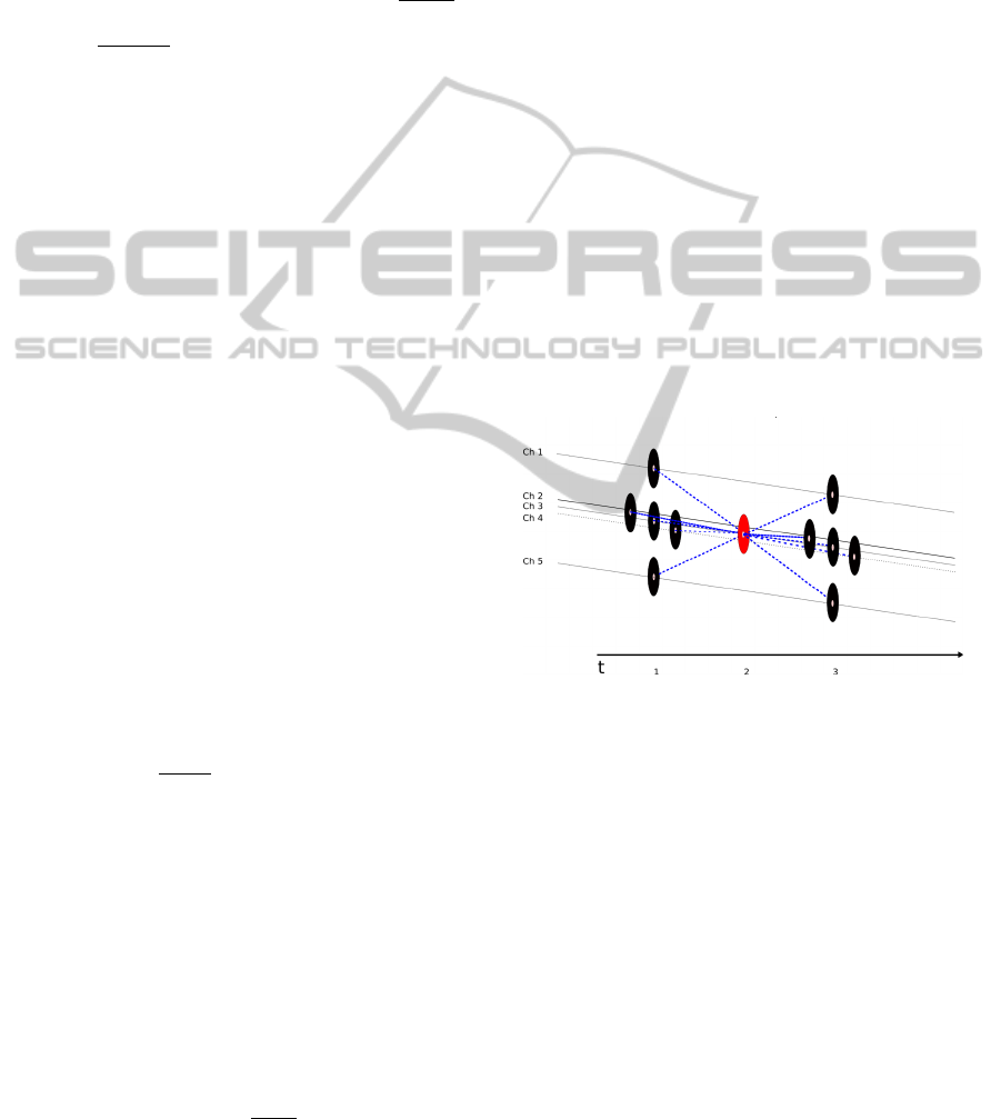
Figure 2: Detail of the graph after the even/odd split for the
static approach. The even element (in red) is linked to the
surrounding odd elements (in black) adding spatial infor-
mation to the decomposition.
• Graph lifting scheme and mutual information
driven graph building.
Each detail and approximation coefficient sets
from the different temporal segments were classified
with a separate LDA model after applying CSP. This
led to a total of n
s
∗l ∗2 LDA outputs, with n
s
being
the number of segments and l the number of levels. A
majority voting approach was carried out in order to
obtain the final classification output for each trial.
A cross-validation step using five folds was per-
formed over the training data in order to select the
two free parameters involved: the threshold applied to
the mutual information matrix in Section 2.3 and the
number of CSP features as explained in Section 2.4.
PhyCS2014-InternationalConferenceonPhysiologicalComputingSystems
8
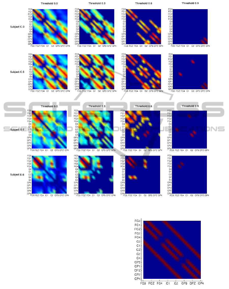
Figure 3: Representation of the values of M for subjects C-3 and C-5 applying different thresholds.
Figure 4: Representation of the values of matrix M for subjects E-7 and E-8 applying different thresholds.
3 RESULTS AND DISCUSSION
From the analysis of the mutual information matrix
M for the different subjects we learn that, in general,
the standard deviations of the paired calculation do
not differ much when compared among classes (two
orders of magnitude smaller than the mean). There-
fore, instead of computing a matrix M and a different
graph to process one class against the others, we just
use the whole set of data to generate the mutual infor-
mation based adjacency matrix. This simplifies the
model decreasing the execution time. It is also note-
worthy that the performance of the transform calcu-
lation does not vary although the values of the filters
applied changed.
Figure 3 and Figure 4 are graphical representa-
tions of the values of the matrix M for different users
Figure 5: Values of the matrix M for the static graph ap-
proach.
and with different thresholds. In Figure 3 we find two
examples to show that there exists a clear correlation
MultiresolutionAnalysisofanInformationbasedEEGGraphRepresentationforMotorImageryBrainComputerInterfaces
9
between the electrode spatial location and the mutual
information, the parallel lines crossing the figure di-
agonally corresponds to high mutual information val-
ues between adjacent electrodes. This correlation is
more evident if we compare it with with Figure 5,
which corresponds to the matrix M of the static ap-
proach. Although in Figure 4 this effect is still notice-
able, it is more obvious how, for these specific sub-
jects, the inter-electrode information is more promi-
nent in particular locations of the motor cortex, con-
cretely, in the frontal and central lobes for subject E-7
and eminently central for subject E-8.
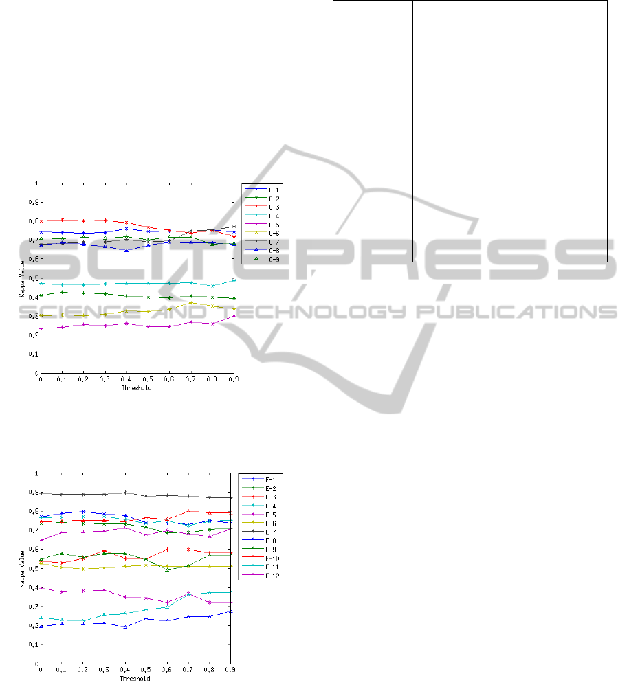
Figure 6: Median of the Kappa value in function of the
threshold applied to the matrix M for the competition
dataset.
Figure 7: Median of the Kappa value in function of the
threshold applied to the matrix M for the Essex dataset.
After applying the experimental methodology de-
scribed in Section 2.5 we can analyse the impact of
the automatic graph building on the classification re-
sults. Figure 6 and Figure 7 show how the median
Kappa values change when different threshold val-
ues are applied. It is clear that the behaviour of the
Table 1: Results on the Essex dataset in terms of Kappa
values. The mean accuracy is included at the bottom.
Subject GLS GLS + Mutual Information
E-1 0.757 0.741
E-2 0.736 0.744
E-3 0.539 0.644
E-4 0.730 0.712
E-5 0.392 0.393
E-6 0.529 0.488
E-7 0.883 0.891
E-8 0.210 0.263
E-9 0.565 0.581
E-10 0.757 0.774
E-11 0.237 0.321
E-12 0.648 0.707
Mean Kappa 0.582 0.605
± ±
0.21 0.19
Mean Acc 0.723 0.737
± ±
0.14 0.13
method is dependant on the subject of analysis. Some
subjects, such as E-8, C-4 and C-2, are not signifi-
cantly affected by the change of the threshold value,
although, on the other hand, we find subjects where
the Kappa value fluctuates around 0.1 depending on
the threshold value such as in subjects C-3, C-7, E-9
and E-11.
After selecting the two parameters, the mutual in-
formation threshold and the number of features used
in CSP, from the cross-validation results we can com-
pute the classification performance on the evaluation
data. Table 1 shows the Kappa values and mean accu-
racy for the Essex dataset and Table 2 for the compe-
tition dataset.
For 80% of the 21 subjects the proposed method
achieved a higher Kappa value. For some of the sub-
jects this improvement rises the Kappa value by 0.1
when compared to the static approach. In order to
obtain enough data to perform a significance test we
repeated the experiments by joining the validation and
evaluation datasets for each subject and then perform-
ing a cross-validation with five folds.
As a final remark we can mention that the pro-
posed method obtains a Kappa value of 0.586 using
the competition dataset, while the winner achieved
0.57. The small number of subjects in the competi-
tion data does not allow us to carry out a definitive
significance test to compare both approaches.
4 CONCLUSIONS
In this study we have proposed a novel method to
improve the EEG data representation based on static
PhyCS2014-InternationalConferenceonPhysiologicalComputingSystems
10

Table 2: Results on the competition dataset in terms of
Kappa values. The mean accuracy is included at the bot-
tom.
Subject GLS GLS + Mutual Information
C-1 0.754 0.763
C-2 0.410 0.419
C-3 0.800 0.805
C-4 0.484 0.475
C-5 0.243 0.257
C-6 0.317 0.364
C-7 0.629 0.758
C-8 0.661 0.707
C-9 0.698 0.721
Mean Kappa 0.555 0.586
± ±
0.19 0.20
Mean Acc 0.666 0.689
± ±
0.15 0.15
graphs by using the mutual information among the
different channels. This new strategy for building the
graph also has an impact on the filter design, allowing
an automatic way to weight the contribution of the
different spatial locations.
Comparing the mutual information matrices from
different subjects we can observe how the initial static
graph approach, where the surrounding electrodes
were linked together, was appropriate as close elec-
trodes tend to share similar information.
After applying the proposed methodology on the
two data sets Kappa value was increased for an 80%
percent of the subjects obtaining for several subjects
an improvement of 0.1 in their Kappa value.
The present study is also an example of the possi-
bilities offered by the lifting transform, where MRA
approaches can be easily implemented without the in-
herent complexity of the first generation wavelets.
The positive results presented hereby encourage
us to explore new ways for optimising the graph rep-
resentation of EEG data. Although mutual infor-
mation has helped to improve the classification rate,
other techniques such as Granger causality or phase
synchronisation indexes, which are more robust when
coping with non-stationarity, should be examined in
future work.
ACKNOWLEDGEMENTS
The first author would like to thank the EPSRC for
funding his Ph.D. study via an EPSRC DTA award.
REFERENCES
Allison, B., Graimann, B., and Grser, A. (2008). Why use a
BCI if you are healthy. Proceedings of BRAINPLAY,
playing with your brain.
Asensio-Cubero, J., Gan, J. Q., and Palaniappan, R. (2013).
Multiresolution analysis over simple graphs for brain
computer interfaces. Journal of Neural Engineering,
10(4):046014.
Blankertz, B., Muller, K. R., Krusienski, D. J., Schalk, G.,
Wolpaw, J. R., Schlogl, A., Pfurtscheller, G., Millan,
J. R., Schroder, M., and Birbaumer, N. (2006). The
BCI competition III: validating alternative approaches
to actual BCI problems. IEEE Transactions on Neural
Systems and Rehabilitation Engineering, 14(2):153–
159.
Brunner, C., Leeb, R., Muller-Putz, G. R.,
Schlogl, A., and Pfurtscheller, G. (2008).
BCI competition 2008 - Graz data set A.
http://www.bbci.de/competition/iv/desc 2a.pdf.
Carrera-Leon, O., Ramirez, J. M., Alarcon-Aquino, V.,
Baker, M., D’Croz-Baron, D., and Gomez-Gil, P.
(2012). A motor imagery bci experiment using
wavelet analysis and spatial patterns feature extrac-
tion. In Engineering Applications (WEA), 2012 Work-
shop on, pages 1–6. IEEE.
Claypoole Jr, R. L., Baraniuk, R. G., and Nowak, R. D.
(1998). Adaptive wavelet transforms via lifting. In
Proceedings of IEEE International Conference on
Acoustics, Speech and Signal Processing, volume 3,
pages 1513–1516.
Cohen, J. (1960). A coefficient of agreement for nominal
scales. Educational and Psychological Measurement,
20(1):37–46.
Cover, T. M. and Thomas, J. A. (2012). Elements of Infor-
mation Theory. John Wiley & Sons.
Daubechies, I. (2006). Ten Lectures on Wavelets. Society
for Industrial and Applied Mathematics.
Dornhege, G. (2007). Toward Brain-Computer Interfacing.
The MIT Press.
Mallat, S. G. (1989). A theory for multiresolution sig-
nal decomposition: The wavelet representation. IEEE
Transactions on Pattern Analysis and Machine Intel-
ligence., 11(7):674–693.
Martinez-Enriquez, E. and Ortega, A. (2011). Lifting trans-
forms on graphs for video coding. In Data Compres-
sion Conference, pages 73–82. IEEE.
Narang, S. K. and Ortega, A. (2009). Lifting based wavelet
transforms on graphs. In Conference of Asia-Pacific
Signal and Information Processing Association, pages
441–444.
Peng, H., Long, F., and Ding, C. (2005). Feature se-
lection based on mutual information criteria of max-
dependency, max-relevance, and min-redundancy.
Pattern Analysis and Machine Intelligence, IEEE
Transactions on, 27(8):1226–1238.
Perseh, B. and Sharafat, A. R. (2012). An efficient p300-
based bci using wavelet features and ibpso-based
channel selection. Journal of Medical Signals and
Sensors, 2(3):128.
MultiresolutionAnalysisofanInformationbasedEEGGraphRepresentationforMotorImageryBrainComputerInterfaces
11

Pfurtscheller, G. and Lopes da Silva, F. H. (1999). Event-
related EEG/MEG synchronization and desynchro-
nization: basic principles. Clinical Neurophysiology,
110(11):1842–1857.
Ramoser, H., Muller-Gerking, J., and Pfurtscheller, G.
(2000). Optimal spatial filtering of single trial eeg dur-
ing imagined hand movement. IEEE Transactions on
Rehabilitation Engineering, 8(4):441–446.
Schrder, P. and Sweldens, W. (1995). Spherical wavelets:
Efficiently representing functions on the sphere. In
Proceedings of the 22nd Annual Conference on Com-
puter Graphics and Interactive Techniques, pages
161–172. ACM.
Shen, G. and Ortega, A. (2008). Comopact image repre-
sentation using wavelet lifting along arbitrary trees.
In 15th IEEE International Conference on Image Pro-
cessing, 2008. ICIP 2008., pages 2808–2811. IEEE.
Sweldens, W. (1996). Wavelets and the lifting scheme: A
5 minute tour. Zeitschrift fur Angewandte Mathematik
und Mechanik, 76(2):41–44.
Sweldens, W. (1998). The lifting scheme: A construction of
second generation wavelets. SIAM Journal on Mathe-
matical Analysis, 29(2):511.
Sweldens, W. and Schrder, P. (2000). Building your own
wavelets at home. Wavelets in the Geosciences, pages
72–107.
PhyCS2014-InternationalConferenceonPhysiologicalComputingSystems
12
