Classifying and Visualizing Motion Capture Sequences
using Deep Neural Networks
Kyunghyun Cho and Xi Chen
Department of Information and Computer Science, Aalto University School of Science, Espoo, Finland
Keywords:
Gesture Recognition, Motion Capture, Deep Neural Network.
Abstract:
The gesture recognition using motion capture data and depth sensors has recently drawn more attention in
vision recognition. Currently most systems only classify dataset with a couple of dozens different actions.
Moreover, feature extraction from the data is often computational complex. In this paper, we propose a novel
system to recognize the actions from skeleton data with simple, but effective, features using deep neural
networks. Features are extracted for each frame based on the relative positions of joints (PO), temporal differ-
ences (TD), and normalized trajectories of motion (NT). Given these features a hybrid multi-layer perceptron
is trained, which simultaneously classifies and reconstructs input data. We use deep autoencoder to visualize
learnt features. The experiments show that deep neural networks can capture more discriminative information
than, for instance, principal component analysis can. We test our system on a public database with 65 classes
and more than 2,000 motion sequences. We obtain an accuracy above 95% which is, to our knowledge, the
state of the art result for such a large dataset.
1 INTRODUCTION
Gesture recognition has been a hot and challenging
research topic for several decades. There are two
main kinds of source data: video and motion cap-
ture data (Mocap). Mocap records the human actions
based on the human skeleton information. Its classifi-
cation is very important in computer animation, sports
science, human–computer interaction (HCI) and film-
making.
Recently the low cost and high mobility of RGB-
D sensors, such as Kinect, have become widely
adopted by the game industry as well as in HCI. Espe-
cially in computer vision, the gesture recognition us-
ing data from the RGB-D sensors is gaining more and
more attention. However,the computational difficulty
in directly processing 3–D cloud data from depth in-
formation often leads to utilizing the human skeleton
extracted from the depth information (Shotton et al.,
2011) instead.
However, conventional recognition systems are
mostly applied on a small dataset with a couple of
dozens different actions, which is often the limitation
imposed by the design of a system. Conventional de-
signs may be classified into two categories: a whole
motion is represented by one feature matrix or vector
(Raptis et al., 2011), and classified by a classifier as a
whole (M¨uller and Roder, 2006); or a library of key
features (Wang et al., 2012) is learned from the whole
dataset, and then each motion is represented as a bag
or histogram of words (Raptis et al., 2008) or a path
in a graph (Barnachon et al., 2013).
In the first type of system, principal component
analysis (PCA) is often used to form equal-size fea-
ture matrices or vectors from variable-length motion
sequences (Zhao et al., 2013; Vieira et al., 2012).
However, due to a large number of inter- and intra-
class variations among motions, a single feature ma-
trix or vector is likely not enough to capture important
discriminativeinformation. This makes these systems
inadequate for a large dataset.
The second type of system decomposes a motion
with a manual setup sliding window or key features
(Raptis et al., 2008) and builds a codebook by cluster-
ing (Chung and Yang, 2013). These approaches also
suffer from a large number of action classes due to
a potentially excessive size of codebook, in the case
of using a classifier such as support vector machines
(Ofli et al., 2013) as well as an overly complicated
structure, if one tries to build a motion graph.
In this paper, we recognize actions from skele-
ton data with two major contributions: (1) we pro-
pose to build the recognition system based on joint
distribution model of the per-frame feature set con-
122
Cho K. and Chen X..
Classifying and Visualizing Motion Capture Sequences using Deep Neural Networks.
DOI: 10.5220/0004718301220130
In Proceedings of the 9th International Conference on Computer Vision Theory and Applications (VISAPP-2014), pages 122-130
ISBN: 978-989-758-004-8
Copyright
c
 2014 SCITEPRESS (Science and Technology Publications, Lda.)

0
20
40
60
−200
−150
−100
−50
0
50
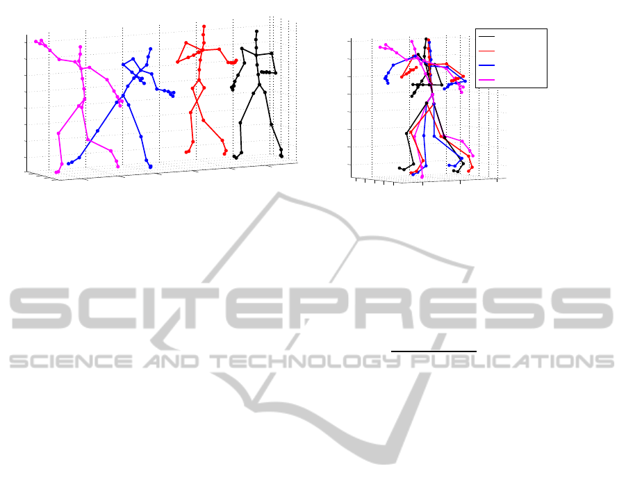
(a) Original
−40
−20
0
20
40
−50
0
50
−80
−60
−40
−20
0
20
40
60
frame:30
frame:90
frame:150
frame:200
(b) Root
Figure 1: A throwFar action in (a) original and (b) root coordinates.
taining information of the relative positions of joints,
their temporal difference and the normalized trajec-
tory of the motion; (2) we propose a novel variant of
a multi-layer perceptron, called a hybrid MLP, that si-
multaneously classifies and reconstructs the features,
which outperforms a regular MLP, extreme learning
machines (ELM) as well as SVM; meanwhile a deep
autoencoder is trained to visualize the features in 2-
dimensional space, comparing with PCA using the
two leading principal components, we clearly see that
autoencoder can extract more distinctive information
from features. We test our system on a publicly avail-
able database containing 65 action classes and more
than 2,000 motions with above 95% accuracy.
2 FEATURE EXTRACTION
In this section we describe how to extract the pro-
posed features from each frame. Fig. 1 (a) shows
some frames from a motion sequence throwfar. Since
the original coordinates are dependent on a performer
and the space to which the performer belongs, those
coordinates are not directly comparable between dif-
ferent performers even if they all perform the same
action. Hence, we normalize the orientation such
that each and every skeleton has its root at the ori-
gin (0, 0, 0) with the same orientation matrix of iden-
tity. For example, Fig. 1 (b) shows the orientation-
normalized versions of the skeleton in Fig. 1 (a). We
further normalize the length of all connected joints to
be 1 to make them independent of a performer. The
concatenation of 3D coordinates of joints forms the
feature (PO), which describes relative relationships
among the joints.
Some actions are similar to each other in a frame-
level. For instance, the actions of standing up and
sitting down are just reverse in time but with almost
identical frames, which results in almost identical PO
features for corresponding frames in those actions.
Hence, we compute the temporal differences (TD) be-
tween pairs of PO feature by
f
i
TD
=



f
i
PO
1 ≤ i < m

f
i
PO
− f
i−m+1
PO

||f
i
PO
− f
i−m+1
PO
||
m ≤ i ≤ N ,
(1)
where f
i
PO
and m are the PO feature vector at the i-th
frame and the temporal offset (1 < m < N), respec-
tively. TD feature preserves the temporal relationship
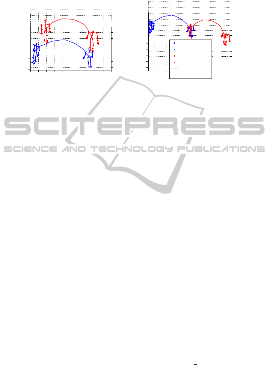
of the same joint. Normalized trajectory (NT) extracts
the absolute trajectory of the motion. Fig.2(a) shows
two motions: walk in a left circle and walk in a right
circle. However, in this figure the trajectories of left
circle and right circle are not distinguishable. In or-
der to incorporate the trajectory information, we set
the same orientation and starting position for the root
in the first frame and use a relative position of the root
of all the rest frames in the motion sequences from the
initial frame, normalized into [−1, 1] in each dimen-
sion. See Fig. 2 (b) for the effect of this transforma-
tion. The final feature for each frame is a concatena-
tion of three features. The dimension of the feature is
3× n× 2 + 3, where n is the number of joints in use
in PO.
For skeleton extracted from RGB-D sensor, often
the rotation matrix and translation vector related with
the joints are not available. In this case any skele-
ton can be selected as a stardard template frame, the
rotation matrix between the other skeletons and the
template can be calculated as in (Chen and Koskela,
2013). In the similar way the features from skeleton
data with only 3D joint coordinates can be extracted.
ClassifyingandVisualizingMotionCaptureSequencesusingDeepNeuralNetworks
123

−200 −150 −100 −50 0 50 100 150 200 250 300
−150
−100
−50
0
50
100
150
0
50
100
150
z
x
y
(a) Original
−300 −200 −100 0 100 200 300
−150
−100
−50
0
50
100
150
200
−200
−100
0
100
200
z
x
y
Start walk left
Stop walk left
Start walk right
Stop walk right
Trajectory Left
Trajectory right
(b) Transformed
Figure 2: Trajectories of two different walks in (a) original and (b) transformed coordinates.
3 DEEP NEURAL NETWORKS:
MULTI-LAYER PERCEPTRONS
A multi-layer perceptron (MLP) is a type of deep neu-
ral networks that is able to perform classification (see,
e.g., (Haykin, 2009)). An MLP can approximate any
smooth, nonlinear mapping from a high dimensional
sample to a class through multiple layers of hidden
neurons.
The output or prediction of an MLP having L hid-
den layers and q output neurons given a sample x is
typically computed by
u(x | θ) = (2)
σ

U
⊤
φ

W
⊤
[L]
φ

W
⊤
[L−1]
···φ

W
⊤
[1]
x

···

,
where σ and φ are component-wise nonlinear func-
tions, and θ =

U, W
[1]
, . . . , W
[L]

is a set of parame-
ters. We have omitted a bias without loss of general-
ity. A logistic sigmoid function is usually used for the
last nonlinear function σ. Each output neuron corre-
sponds to a single class.
Given a training set
n
x
(n)
, y
(n)
o
N
n=1
, an MLP
is trained to approximate the posterior probability
p(y
j
= 1 | x) of each output class y
j
given a sample x
by maximizing the log-likelihood
L
sup
(θ) =
N
∑
n=1
q
∑
j=1

y
(n)
j
logu
j

x
(n)

+

1− y
(n)
j

log

1− u
j

x
(n)

, (3)
where a subscript j indicates the j-th component. We
omitted θ to make the above equation uncluttered.
Training can be efficiently done by backpropagation
(Rumelhart et al., 1986).
3.1 Hybrid Multi-layer Perceptron
It has been noticed by many that it is not trivial to
train deep neural networks to have a good general-
ization performance (see, e.g., (Bengio and LeCun,
2007) and references therein), especially when there
are many hidden layers between input and output lay-
ers. One of promising hypotheses explaining this dif-
ficulty is that backpropagation applied on a deep MLP
tends to utilize only a few top layers (Bengio et al.,
2007). A method of layer-wise pretraining has been
proposed to overcome this problem by initializing the
weights in lower layers with unsupervised learning
(Hinton and Salakhutdinov, 2006).
Here, we propose another strategy that forces
backpropagation algorithm to utilize lower layers.
The strategy involves training an MLP to classify and
reconstruct simultaneously by training a deep autoen-
coder with the same set of parameters, except for the
weights between the penultimate and output layers to
reconstruct an input sample as well as possible.
A deep autoencoder is a symmetric feedforward
neural network consisting of an encoder
h = f(x) = f
[L−1]
◦ f
[L−2]
◦ · ·· ◦ f
[1]
(x)
and a decoder
˜
x = g(x) = g
[2]
◦ · ·· ◦ g
[L−1]
(h),
where
f
[l]
(s
[l−1]
) = φ

W
⊤
[l]
s
[l−1]

,
g
[l]
(s
[l+1]
) = ϕ

W
[l]
s
[l+1]

.
φ and ϕ are component-wise nonlinear functions.
The parameters of a deep autoencoder is estimated
by maximizing the negative squared difference which
is defined to be
L
unsup
(θ) = −
1
2
N
∑
n=1



x
(n)
−
˜
x
(n)



2
2
. (4)
VISAPP2014-InternationalConferenceonComputerVisionTheoryandApplications
124

Our proposed strategy combines these two net-
works while sharing a single set of parameters θ by
optimizing a weighted sum of Eq. (3) and Eq. (4):
L (θ) = (1 − λ)L
sup
(θ) + λL
unsup
(θ), (5)
where λ ∈ [0, 1] is a hyperparameter. When λ is 0, the
trained model will be purely an MLP, while it will be
an autoencoder if λ = 1. We call an MLP that was
trained with this strategy with non-zero λ a hybrid
MLP
1
.
There are two advantages in the proposed strat-
egy. First, the weights in lower layers naturally have
to be utilized, since those weights must be adapted to
reconstruct an input sample well. This may further
help achieving a better classification accuracy simi-
larly to the way unsupervised layer-wise pretraining
which also optimized the reconstruction error , in the
case of using autoencoders, helps obtaining a better
classification accuracy on novel samples. Secondly,
in this framework, it is trivial to use vast amount of
unlabeled samples in addition to labeled samples. If
stochastic backpropagation is used, one can compute
the gradients of L by combining the gradients of L
sup
and L
unsup
separately using separate sets of labeled
and unlabeled samples.
4 CLASSIFYING AN ACTION
SEQUENCE
An action sequence is composed of an certain amount
of frames. We use a multi-layer perceptron to model a
posterior distribution of classes given each frame. Let
us define s
c
∈ {0, 1} be a binary indicator variable. If
s
c
is one, the sequence belongs to the action c, and
otherwise, belongs to another action. Since each se-
quence consists of N ≥ 1 frames, let us further define
f
i,c
∈ {0, 1} as a binary variable indicating whether
the i-th frame belongs to the action c.
When a given sequence s = (f
1
, f
2
, . . . , f
N
) is of an
action c, every frame f
i
in the sequence is also of an
action c. In other words, if s
c
= 1, f
i,c
= 1 for all i. So,
we may check the joint probability of all frames in the
sequence to determine the action of the sequence:
p(s
c
= 1 | s) = (6)
p( f
1,c
= 1, f
2,c
= 1, . . . , f
N,c
= 1 | f
1
, f
2
, . . . , f
N
).
In this paper, we assume temporal independence
among the frames in a single sequence, which means
that the class of each frame depends only on the fea-
tures of the frame. Then, Eq. (6) can be simplified
1
A similar approach was proposed in (Larochelle and
Bengio, 2008) in the case of restricted Boltzmann machines.
into
p(s
c
= 1 | s) =
N
∏
i=1
p( f
i,c
= 1 | f
i
). (7)
With this assumption, the problem of gesture
recognition is reduced to first train a classifier to per-
form frame-level classification and then to combine
the output of the classifier according to Eq. (7). A
multi-layer perceptron which approximates the poste-
rior probability distribution over classes by Eq. (2) is
naturally suited to this approach.
5 EXPERIMENTS
In the experiment we tried to evaluate the perfor-
mance of our proposed recognition system through a
public dataset. We assessed the performance of deep
neural networks including regular and hybrid MLP by
comparing them against extreme learning machines
(ELM) and support vector machines (SVM). The ef-
fectiveness of the feature set was evaluated by the
classification accuracy and the visualization in 2D
space by deep autoencoders.
5.1 Dataset
The Motion Capture Database HDM05 (M¨uller et al.,
2007) is a well organized large MOCAP dataset. It
provides a set of short cut MOCAP clips, and each
clip contains one integral motion. In the original
dataset, there are 130 gesture groups. However, there
are some gestures that essentially belong to a single
class. For instance, walk 2 steps and walk 4 steps be-
long to a single action walk. Hence, we combined
some of the classes based on the following rules:
1. Motions repeating with different times are com-
bined into one action.
2. Motions with the only difference of the starting
limb are combined into one action.
After the reorganizationthe whole dataset consist-
ing of 2,337 motion sequences and 613,377 frames is
divided into 65 actions
2
.
5.2 Settings
We used 10-fold cross validation to assess the perfor-
mance of a classifier. The data was randomly split into
10 balanced partitions of sequences. PO feature was
formed by 5 joints:head, hands and feet. The param-
eter m in TD was set as 0.3 second interval between
2
See the appendix for the complete list of 65 actions
ClassifyingandVisualizingMotionCaptureSequencesusingDeepNeuralNetworks
125

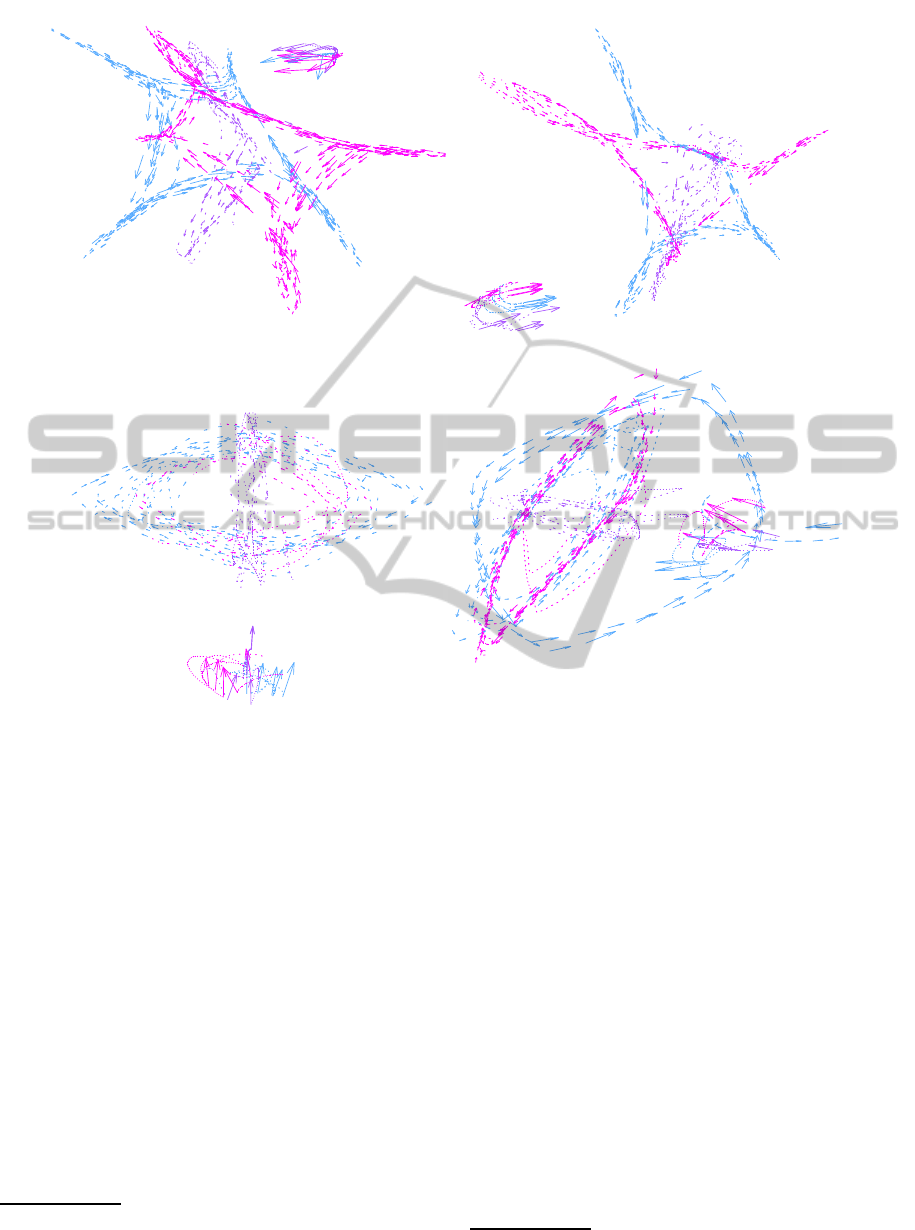
(a) DNN (PO+TD) (b) DNN (PO+TD+NT)
(c) PCA (PO+TD) (d) PCA (PO+TD+NT)
Figure 3: Visualization of actions rotateArmsRBackward (blue), rotateArmsBothBackward (purple) and rotateArmsLBack-
ward (red). Each arrow denotes the direction and magnitude of change in the latent space. Five randomly selected sequences
per action are shown.
frames. The total dimension of the feature vector is
33. To test the distinctiveness of the features, we re-
ported the classification accuracy for each frame, and
evaluated the system performance by the accuracy of
each sequence. The standard deviations were also cal-
culated for 10-fold cross validation.
We trained deep neural networks having two hid-
den layers of sizes 1000 and 500 with rectified linear
units
3
. A learning rate was selected automatically by
a recently proposed ADADELTA (Zeiler, 2012). Usu-
ally the optimal λ can be selected by the validation set
and on a grid search. To illustrate the influences of λ
in hybrid MLP, we selected four different values for
λ: 0, 0.1, 0.5 and 0.9. The parameters were simply
initialized randomly, and no pretraining strategy was
used
4
.
3
The activation of a rectified linear unit is max(0, α),
where α is the input to the unit.
4
We used a publicly available MATLAB toolbox
When a tested classifier outputs the posterior
probabilityof a class given a frame, we chose the class
of a sequence by
argmax
c
N
∑
i=1
log p( f
i,c
= 1 | f
i
)
based on Eq. (7). If a classifier does not return a prob-
ability but only the chosen class, we used a simple
majority voting.
As a comparison, we tried an extreme learning
machine (ELM) (Huang et al., 2006) and SVM in
the same system. We used 2,000 hidden neurons
for ELM. For SVM we used a radial-basis function
kernel, and the hyperparameters C and γ were found
through a grid-search and cross-validation.
deepmat for training and evaluating deep neural networks:
https://github.com/kyunghyuncho/deepmat
VISAPP2014-InternationalConferenceonComputerVisionTheoryandApplications
126

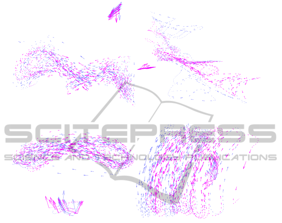
(a) DNN (PO+TD)
(b) DNN (PO+TD+NT)
(c) PCA (PO+TD) (d) PCA (PO+TD+NT)
Figure 4: Visualization of actions jogLeftCircle (blue) and jogRightCircle (purple). Each arrow denotes the direction and
magnitude of change in the latent space. Ten randomly chosen sequences per action were visualized.
5.3 Qualitative Analysis: Visualization
In order to have a better understanding of what a deep
neural network learns from the features, we visualized
the features using a deep autoencoder with two linear
neurons in the middle layer (Hinton and Salakhutdi-
nov, 2006). The deep autoencoder had three hidden
layers of size 1000, 500 and 100 between the input
and middle layers. It should be noted that no label in-
formation was used to train these deep autoencoders.
In the experiment, we trained two deep autoencoders
using with and without the normalized trajectories
(NT) to see what the relative feature (PO+TD) pro-
vides to the system and the impact of the absolute
feature. Since in previous works PCA has been of-
ten used for dimensionality reduction of motion fea-
tures, we also tried to visualize features using the two
leading principal components.
In Fig. 3, we visualized three distinct, but very
similar, actions; rotateArmsRBackward, rotateArms-
BothBackward and rotateArmsLBackward. These ac-
tions in the figure were clearly distinguishable when
the deep autoencoder was used. However, rotateArm-
sRBackward and rotateArmsLBackward were not dis-
tinguishable at all when only the PO and TD features
were used by PCA (see Fig. 3 (c)). Even when all
three features (PO+TD+NT) were used, the visualiza-
tion by PCA did not help distinguishing these actions
clearly.
In Fig. 4, two actions, jogLeftCircle and jogRight-
Circle, were visualized. When only PO and TD fea-
tures were used, neither the deep autoencoder nor
PCA was able to capture differences between those
actions. However, the deep autoencoder was able to
distinguish those actions clearly when all three pro-
posed features were used (see Fig. 4 (b)).
The former visualization shows that a deep neu-
ral network with multiple nonlinear hidden layers can
ClassifyingandVisualizingMotionCaptureSequencesusingDeepNeuralNetworks
127

Table 1: Classification accuracies. Standard deviations are shown inside brackets. The highest accuracy in each row is marked
bold.
Feature
Hybrid MLP
Set ELM SVM MLP λ = 0.1 0.5 0.9
PO+TD 70.40% (1.32) 83.82% (0.79) 84.35% (0.91) 84.39% (0.87) 84.57% (1.56) 84.23% (1.27)
PO+TD+NT 74.28% (1.56) 87.06% (0.82) 87.42% (1.43) 87.96% (1.38) 87.34% (0.66) 87.28% (1.38)
Feature
Hybrid MLP
Set ELM SVM MLP λ = 0.1 0.5 0.9
PO+TD 91.57% (0.88) 94.95% (0.82) 95.20% (1.38) 95.46% (0.99) 95.59% (0.76) 95.55% (1.14)
PO+TD+NT 92.76% (1.53) 95.12% (0.58) 94.86% (0.99) 95.21% (0.86) 94.82% (1.17) 95.04% (0.86)
learn more discriminative structure of data. Further-
more, according to the latter visualization, we can see
that the normalized trajectories help distinguish loco-
motions with different traces, however, with only a
powerful model as a deep neural network. Through
the experiment we could see that deep neural net-
works are able to learn highly discriminative infor-
mation from our features of motion.
5.4 Quantitative Analysis: Recognition
In Tab. 1, the frame-level accuracies obtained by var-
ious classifiers with two different sets of features can
be found. We can see that the NT feature clearly in-
creases the classification accuracy around 3− 4% for
all the classifiers. Comparing the different classifiers,
we can see that the MLPs were able to obtain signif-
icantly higher accuracies than the ELM and perform
slightly better than SVM. Furthermore, although it is
not clearly significant statistically, we can see that a
hybrid MLP often outperforms the regular MLP with
a right choice of λ.
A similar trend of the MLPs outperforming the
other classifiers could be observed also in sequence-
level performance shown in Tab. 1. Again in the
sequence-levelclassification, we observedthat the hy-
brid MLP with a right choice of λ marginally out-
performed the regular MLP, and it also outperformed
SVM and ELM. For both frame-level and sequence-
level accuracy, the highest accuracy for PO+TD fea-
tures is from hybrid MLP with λ = 0.5 and for the
whole feature set with λ = 0.1.
However, the classification accuracies ob-
tained using the two sets of features (PO+TD vs
PO+TD+NT) are very close to each other. Compared
to the 3 − 4% differences in the classification for
each frame, the differences between the performance
obtained using the two sets are within the standard
deviations. Even though NT feature increases the
frame accuracy significantly it did not have the same
effect on the sequence level. One potential reason is
that once a certain level of frame level recognition is
achieved, the sequence level performance using our
posterior probability model saturates.
6 CONCLUSIONS
In this paper, we proposed a gesture recognition sys-
tem using multi-layer perceptrons for recognizing
motion sequences with novel features based on rel-
ative joint positions (PO), temporal differences (TD)
and normalized trajectories (NT).
The experiments with a large motion capture
dataset (HDM05) revealed that (hybrid) multi-layer
perceptrons could achieve higher recognition rate
than there is the other classifiers could, for 65 classes
with an accuracy of above 95%. Furthermore, the
visualization of feature set of the motion sequences
by deep autoencoders showed the effectiveness of the
proposed feature sets and enabled us to study what
deep neural networks learned. Interestingly, a power-
ful model like a deep neural network combined with
an informative feature set was able to capture the dis-
criminative structure of motion sequences, which was
confirmed by both the recognition and visualization
experiments. This suggests that a deep neural network
is able to extract highly discriminative features from
motion data.
One limitation of our approach is that temporal in-
dependence was assumed when combining the per-
frame posterior probabilities in a sequence. In fu-
ture it will be interesting to investigate possibilities
of modeling temporal dependence.
ACKNOWLEDGEMENTS
This work was funded by Aalto MIDE programme
(project UI-ART), Multimodally grounded language
technology (254104) and Finnish Center of Excel-
lence in Computational Inference Research COIN
(251170) of the Academy of Finland.
VISAPP2014-InternationalConferenceonComputerVisionTheoryandApplications
128

REFERENCES
Barnachon, M., Bouakaz, S., Boufama, B., and Guillou, E.
(2013). A real-time system for motion retrieval and
interpretation. Pattern Recognition Letters.
Bengio, Y., Lamblin, P., Popovici, D., and Larochelle, H.
(2007). Greedy layer-wise training of deep networks.
In Sch¨olkopf, B., Platt, J., and Hoffman, T., editors,
Advances in Neural Information Processing Systems
19, pages 153–160. MIT Press, Cambridge, MA.
Bengio, Y. and LeCun, Y. (2007). Scaling learning algo-
rithms towards AI. In Bottou, L., Chapelle, O., De-
Coste, D., and Weston, J., editors, Large Scale Kernel
Machines. MIT Press.
Chen, X. and Koskela, M. (2013). Classification of rgb-d
and motion capture sequences using extreme learning
machine. In Proceedings of 18th Scandinavian Con-
ference on Image Analysis.
Chung, H. and Yang, H.-D. (2013). Conditional random
field-based gesture recognition with depth informa-
tion. Optical Engineering, 52(1):017201–017201.
Haykin, S. (2009). Neural Networks and Learning Ma-
chines. Pearson Education, 3rd edition.
Hinton, G. and Salakhutdinov, R. (2006). Reducing the di-
mensionality of data with neural networks. Science,
313(5786):504–507.
Huang, G.-B., Zhu, Q.-Y., and Siew, C.-K. (2006). Extreme
learning machine: Theory and applications. Neuro-
computing, 70(1-3):489–501.
Larochelle, H. and Bengio, Y. (2008). Classification us-
ing discriminative restricted Boltzmann machines. In
Proceedings of the 25th international conference on
Machine learning (ICML 2008), pages 536–543, New
York, NY, USA. ACM.
M¨uller, M. and Roder, T. (2006). Motion templates for
automatic classification and retrieval of motion cap-
ture data. In Proceedings of the Eurographics/ACM
SIGGRAPH symposium on Computer animation, vol-
ume 2, pages 137–146, Vienna, Austria.
M¨uller, M., R¨oder, T., Clausen, M., Eberhardt, B., Kr¨uger,
B., and Weber, A. (2007). Documentation mocap
database HDM05. Technical Report CG-2007-2,
U. Bonn.
Ofli, F., Chaudhry, R., Kurillo, G., Vidal, R., and Bajcsy, R.
(2013). Berkeley mhad: A comprehensive multimodal
human action database. In Applications of Computer
Vision (WACV), 2013 IEEE Workshop on, pages 53–
60.
Raptis, M., Kirovski, D., and Hoppe, H. (2011). Real-
time classification of dance gestures from skeleton
animation. In Proceedings of the 2011 ACM SIG-
GRAPH/Eurographics Symposium on Computer An-
imation, pages 147–156. ACM.
Raptis, M., Wnuk, K., Soatto, S., et al. (2008).
Flexible dictionaries for action classification. In
Proc. MLVMA’08.
Rumelhart, D. E., Hinton, G., and Williams, R. J. (1986).
Learning representations by back-propagating errors.
Nature, 323(Oct):533–536.
Shotton, J., Fitzgibbon, A., Cook, M., Sharp, T., Finocchio,
M., Moore, R., Kipman, A., and Blake, A. (2011).
Real-time human pose recognition in parts from single
depth images. In Proc. Computer Vision and Pattern
Recognition.
Vieira, A., Lewiner, T., Schwartz, W., and Campos, M.
(2012). Distance matrices as invariant features for
classifying MoCap data. In 21st International Confer-
ence on Pattern Recognition (ICPR), Tsukuba, Japan.
Wang, J., Liu, Z., Wu, Y., and Yuan, J. (2012). Mining
actionlet ensemble for action recognition with depth
cameras. In Computer Vision and Pattern Recogni-
tion (CVPR), 2012 IEEE Conference on, pages 1290–
1297. IEEE.
Zeiler, M. D. (2012). ADADELTA: An adaptive learning
rate method. arXiv:
1212.5701 [cs.LG] .
Zhao, X., Li, X., Pang, C., and Wang, S. (2013). Human
action recognition based on semi-supervised discrimi-
nant analysis with global constraint. Neurocomputing,
105(0):45 – 50.
APPENDIX: 65 Actions in HDM05
Dataset
1. cartwheelLHandStart1Reps
cartwheelLHandStart2Reps
cartwheelRHandStart1Reps
2. clap1Reps
clap5Reps
3. clapAboveHead1Reps
clapAboveHead5Reps
4. depositFloorR
5. depositHighR
6. depositLowR
7. depositMiddleR
8. elbowToKnee1RepsLelbowStart
elbowToKnee1RepsRelbowStart
elbowToKnee3RepsLelbowStart
elbowToKnee3RepsRelbowStart
9. grabFloorR
10. grabHighR
11. grabLowR
12. grabMiddleR
13. hitRHandHead
14. hopBothLegs1hops
hopBothLegs2hops
hopBothLegs3hops
15. hopLLeg1hops
hopLLeg2hops
hopLLeg3hops
16. hopRLeg1hops
hopRLeg2hops
hopRLeg3hops
17. jogLeftCircle4StepsRstart
jogLeftCircle6StepsRstart
ClassifyingandVisualizingMotionCaptureSequencesusingDeepNeuralNetworks
129

18. jogOnPlaceStartAir2StepsLStart
jogOnPlaceStartAir2StepsRStart
jogOnPlaceStartAir4StepsLStart
jogOnPlaceStartFloor2StepsRStart
jogOnPlaceStartFloor4StepsRStart
19. jogRightCircle4StepsLstart
jogRightCircle4StepsRstart
jogRightCircle6StepsLstart
jogRightCircle6StepsRstart
20. jumpDown
21. jumpingJack1Reps
jumpingJack3Reps
22. kickLFront1Reps
kickLFront2Reps
23. kickLSide1Reps
kickLSide2Reps
24. kickRFront1Reps
kickRFront2Reps
25. kickRSide1Reps
kickRSide2Reps
26. lieDownFloor
27. punchLFront1Reps
punchLFront2Reps
28. punchLSide1Reps
punchLSide2Reps
29. punchRFront1Reps
punchRFront2Reps
30. punchRSide1Reps
punchRSide2Reps
31. rotateArmsBothBackward1Reps
rotateArmsBothBackward3Reps
32. rotateArmsBothForward1Reps
rotateArmsBothForward3Reps
33. rotateArmsLBackward1Reps
rotateArmsLBackward3Reps
34. rotateArmsLForward1Reps
rotateArmsLForward3Reps
35. rotateArmsRBackward1Reps
rotateArmsRBackward3Reps
36. rotateArmsRForward1Reps
rotateArmsRForward3Reps
37. runOnPlaceStartAir2StepsLStart
runOnPlaceStartAir2StepsRStart
runOnPlaceStartAir4StepsLStart
runOnPlaceStartFloor2StepsRStart
runOnPlaceStartFloor4StepsRStart
38. shuffle2StepsLStart
shuffle2StepsRStart
shuffle4StepsLStart
shuffle4StepsRStart
39. sitDownChair
40. sitDownFloor
41. sitDownKneelTieShoes
42. sitDownTable
43. skier1RepsLstart
skier3RepsLstart
44. sneak2StepsLStart
sneak2StepsRStart
sneak4StepsLStart
sneak4StepsRStart
45. squat1Reps
squat3Reps
46. staircaseDown3Rstart
47. staircaseUp3Rstart
48. standUpKneelToStand
49. standUpLieFloor
50. standUpSitChair
51. standUpSitFloor
52. standUpSitTable
53. throwBasketball
54. throwFarR
55. throwSittingHighR
throwSittingLowR
56. throwStandingHighR
throwStandingLowR
57. turnLeft
58. turnRight
59. walk2StepsLstart
walk2StepsRstart
walk4StepsLstart
walk4StepsRstart
60. walkBackwards2StepsRstart
walkBackwards4StepsRstart
61. walkLeft2Steps
walkLeft3Steps
62. walkLeftCircle4StepsLstart
walkLeftCircle4StepsRstart
walkLeftCircle6StepsLstart
walkLeftCircle6StepsRstart
63. walkOnPlace2StepsLStart
walkOnPlace2StepsRStart
walkOnPlace4StepsLStart
walkOnPlace4StepsRStart
64. walkRightCircle4StepsLstart
walkRightCircle4StepsRstart
walkRightCircle6StepsLstart
walkRightCircle6StepsRstart
65. walkRightCrossFront2Steps
walkRightCrossFront3Steps
VISAPP2014-InternationalConferenceonComputerVisionTheoryandApplications
130