A Method of Weather Recognition based on Outdoor Images
Qian Li, Yi Kong and Shi-ming Xia
College of Meteorology and Oceanography, PLA University of Science and Technology, NanJing, China
Keywords: Outdoor Image, Weather Recognition, Power Spectrum Slop, SVM, Decision Tree.
Abstract: To improve the quality of video surveillance in outdoor and automatic acquire of the weather situations, a
method to recognize weather phenomenon based on outdoor images is presented. There are three features of
our method: firstly, the features, such as the power spectrum slope, contrast, noise and saturation and so on
are extracted, after analysing the effect of weather situations on image; secondly, a decision tree is
constructed in accordance with the distance between the features; thirdly, when every SVM classifier on the
non-leaf node of the decision tree is constructed, some features are selected by assigning the weight. The
experiment results prove that the proposed method can effectively recognize the weather situations in
outdoor.
1 INTRODUCTION
In many outdoor applications for computer vision,
the “bad” weather situations, such as haze, fog, rain,
hail and snow, are involved. And it is urgent to
detect and recognize the various outdoor weather
situations, especially the severe ones. Meanwhile,
the observation of weather situations in meteorology
is still mainly rely on manual, and weather situation
is not exactly the same even within every small
region. Therefore, automatic recognition of the
outdoor weather situation based on image or video
data gets more extensive attention in recent years.
According to the duration and extent of
influence to the video or image, weather situations
can be divided into static or steady weather
situations category and dynamic weather situations
category (Garg, 2004).In Static weather situations
such as sunny, cloudy, fog, smoke, haze and so on,
there is some or more stable particles in the
atmosphere to attenuate and refract the ambient
light, so the impact on image quality of these
phenomena is relatively more stable, mainly for the
blur degradation. Dynamic weather situations, such
as rain, snow, dust storm, hail and so on, make
ambient light attenuation and refraction for the
movement of unstable particles in the atmosphere,
and the image quality degradations caused in these
situations are mainly motion blur, point noise and
movement trace noise. Because of the differences in
imaging process, for example, the influence of the
size of rain and snow, the degradation effect will be
different. So identifying and studying different
dynamic weather phenomena in different
environments and situations is one of the difficulties
in current research.
This paper presents an approach to identify and
classification of weather situations to use existing
surveillance cameras to improve the recognition rate
of outdoor image and resolve the problem of
automatic weather observation. We construct
classifiers with the structure of decision tree by
features extracted from the sample outdoor images
and acquire accurate weather situations classification
results to the images captured by video camera.
2 OUR METHODS OVERVIEW
Weather recognition is a brand-new subject and only
a few of previous work has addressed this issue.
Narasimhan (Narasimhan, 2002; Narasimhan, 2003)
improved the image quality through the
establishment of the physical optics model of the
atmosphere in the fog and rain and other inclement
weather, however their research was mainly based
on the premise of the known current weather, and
did not classify the image automatically. Roser
(Roser, 2008) recognized clear, light rain and heavy
rain weather that exists in the image of driver
assistance systems based on HSI color space
histograms. Yan (Yan, 2009) analyzed the gradient
510
Li Q., Kong Y. and Xia S..
A Method of Weather Recognition based on Outdoor Images.
DOI: 10.5220/0004724005100516
In Proceedings of the 9th International Conference on Computer Vision Theory and Applications (VISAPP-2014), pages 510-516
ISBN: 978-989-758-004-8
Copyright
c
 2014 SCITEPRESS (Science and Technology Publications, Lda.)

and HSV color space histograms of the image data
die vehicle equipment to identify the sunny, rainy
and cloudy combined with road information, but
their research background limited within the range
of intelligent transportation and the acquired image
content was simple and feature selection and
recognition had been fixed. Shen (Shen, 2009) used
SIFT transform to the internet images in the same
scene with the different perspectives, and established
the corresponding illumination model and estimated
the weather according to the angle of light at the
scene, but their model can only recognize sunny and
cloudy weather conditions under the changing
illumination. In the modeling process of the moving
object of traffic surveillance video, Lagorio (Lagorio,
2008) estimated the existence of snow from the
changes of parameters in the mixed of Gaussian
model, and speculate fog according to the blurring of
the video frame in frequency domain spatial, but the
method is easily confused by similar rainfall and
other weather situations.
In order to overcome the problem of the
limitations of feature extraction and recognition in
previous work, we present a weather classification
method based on SVM, which can increase the
identified weather types in the training process and
select appropriate features from the candidate
features according to the effect the characteristics of
weather phenomena. After analyzing the influence
of various weather situations to the image quality,
we extract power spectrum slop, contrast, texture
noise and saturation of images as the candidate
features, and establish a decision-tree-based SVM
classification model. The model having trained can
classify the test images to get the corresponding
weather situations. The common weather situations
including sunny, cloudy, fog and rain are considered
in our method and the process flow is as Fig 1.
Training
Test
Training Images
Decision Tree
Construction
Test Images
Features Extraction
Features Extraction Classifiers
Features Selection
Classifier Result
Figure 1: the Framework of Recognition of Weather.
3 FEATURE EXTRACTION
3.1 Power Spectrum Slope
According to the visual perception, the images under
some inclement weather situations, such as rain, fog
etc, seem to be more blurred than those in fine days,
due to losing some high frequency components. Due
to the different image content, so this image by
extracting the slope of the power spectrum (Liu et al,
2008) information, analysis of various weather
phenomena and the impact of image degradation
effects.
We first compute the power spectrum of an
image I with size N*N by taking the squared
magnitude after Discrete Fourier Transform (DFT).
2
1
(,)
|(,)|
Suv
Iuv
M
N

(1)
where
),( vuI
denotes the Fourier transform image.
Then we represent the two-dimensional frequency in
polar coordinates, i.e.,

sinfu

and

cosfv 
,
and construct
),(

fS
,
f
is the power spectrum
image radius after shifting , and

for the polar
angle, by summing the power spectra S over all
directions

,
),(

fS
, using polar coordinates, can
be approximated by



 ),()( fSfS
(2)
Burton (Burton, 1987) has demonstrated that
)( fS
of most natural images is approximately
decrease exponential with
f
, that is:
()
A
Sf
f


(3)
where
A
is a constant, it is clear from (3) that
)ln(
))(ln(
ln
f
fS
A 
,so it can fit a spline line by
)(ln fS
for different radius to strike the slope

and show in Figure 2. While fitting the line, errors
may be considerable because there are fewer points
in the center of the shifted power spectrum image.
Therefore we adopt
8f
to get better fitting
results.
3.2 Contrast Features
Due to attenuation and refraction of light, the
contrasts of images under different weather
situations are quite different, even in the same scene.
AMethodofWeatherRecognitionbasedonOutdoorImages
511

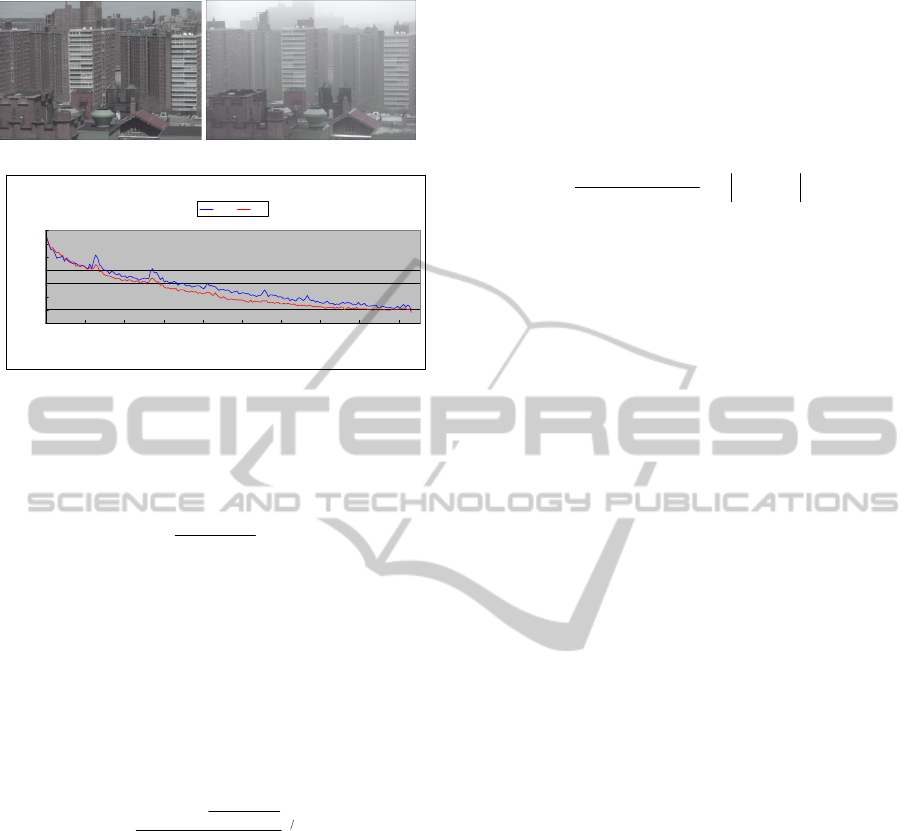
(a) Clear weather image (b) Foggy image
(c) Log Curves of Power Spectrum, with clear
9.2
1

,fog
1.3
2


Figure 2: Analysis of outdoor image power spectrum.
Usually, image contrast is calculated by Mechelson
formula as
max min
max min
L
L
C
L
L



(4)
where
max
L
denotes maximum pixel intensity of the
image, and
min
L is minimum pixel intensity of the
image. While the intensity in image pixels will
dramatic change and cause errors due to the noise
pixel. To increase robustness of contrast estimation,
we get image contrast in different weather situations
by calculating the image intensity standard deviation
(rms) (Peli, 1990)as:
2
(,)
2
(,)
12
()
()
xy
xy
L
L
N
C
N




(5)
where
(,)
x
y
L represents the intensity at in image
(, )
x
y , and N is the number of pixels.
3.3 Noise Features
In dynamic weather situations, the noise point with
different size, shape and trajectory may appear in
image, because there are various types of particles in
the atmosphere and they cause the refraction and
attenuation of light. So we can be effective
extraction of rain, snow and other dynamic weather
phenomena noise features by using fast noise
estimation method (Tai and Yang, 2008). At first a
Laplace noise estimation template is defined as
N .














121
242
121
N
(6)
The noise standard deviation of each point in
image calculates with the template
N and the
average variance of the entire image is defined as:




imageI
yx
NI
HW
),(
)2)(2(6
1

(7)
where
W
represents the image width,
H
is the
image height and
),( yx
I
is the intensity value at the
pixel
),( yx .
3.4 Saturation Features
Though grayscale features are widely used for image
processing tasks that range from low level
algorithms to highly sophisticated modules, there is
growing attention to color information in feature
extraction and tracking. In this paper, we extract
saturation histogram from the HSV color space as
one of classification feature input. In order to make
the approach adapt to different resolution images,
we set histogram as 10 bins and normalize the
histogram results.
4 CLASSIFICATION
Let
F
be the features vector extracted from an
image, and the features of
n
training images consist
of a feature space
{ | 0,1... }
i
SFi n


. Then our
aim is to find a correspondence
:
f
SC
between
the feature space
S and the weather situation set
C
,
in which there is always a weather situation label
()
test
CfF

for any test image feature vector
test
F
.
As SVM method is simple, fast, and powerful,
we use it to learn and classify the weather. In
principle, a SVM generates a hyperplane in the
feature space
S and classifies a test vector by
calculating on which side of the hyperplane the
vector (point) lies. However, SVM classifier is
mainly formulated for a two-class problems and it
can not be directly used for multi-class
classification. According to type of weather features
relatively small, this decision tree based on multi-
class SVM method for classification of weathers.
Log Curves of Power Spectrum
0
2
4
6
8
10
12
14
1
.
6
3
.
2
3
.
8
4
.
2
4
.
4
4
.
7
4
.
8
5
.
0
5
.
1
5
.
2
ln
f
lnS(f
)
Clear Fog
VISAPP2014-InternationalConferenceonComputerVisionTheoryandApplications
512

4.1 Decision Tree
In principle, decision-tree-based SVM method
divides all the classes into n sub-classes (we set n as
2) with a hyperplane, and one or some classes are
separated from remaining classes. In classification,
starting from the top of the decision tree, we
decompose the classes on the node of tree into sub-
classes recursively, until all leaf nodes contains only
one type of class. Then for each non-leaf node in the
decision tree, there should be a SVM as the
classification function. Therefore, we must construct
a binary decision tree at first, as (Takahashi, 2002)
proposed four decision tree constructing methods. In
this paper, we bottom-up construct the decision tree
with the extracted training feature vectors as
follows:
Step 1: Calculate the mean feature vector of the
feature vector set
i
X
for the
ith
class as:



i
Xx
i
x
X
1
i
u
(8)
Then we calculate the Euclidean distance of the
mean vectors between the class
i
and the class
j
.
Because each component in the feature vector is
inconsistent, we normalize Euclidean distance as:



N
i
i
N
1
1
uu
(9)
u
u
u
u
j
i
jiij
dd  )(
(10)
Then all of training samples belong to different
clusters with category center.
Step 2: For the classes which belong to different
clusters, calculate the smallest distance and merge
the associated two classes to the same cluster.
Step 3: Repeat Step 2, until all the classes are
merged into the same node. For the N class problem,
it is usually repeated N-1 times.
Step 4: for each combination in Step 3, a
decision tree node and the corresponding vector
machine function are constructed. if not all of the
node’s child nodes is leaf node, it should continue
merge and establish the vector machines classifier.
4.2 SVM Classifier Construction
After constructing the classification decision tree as
section 4.1, there should be a SVM classifier on each
non-leaf node. In the classification process, different
feature in feature set have different impact to
different SVM classifiers. So we select features
indirectly by weighting features, some features with
greater impact on classification will be set larger
weight, while the features with small impact will be
set smaller weight even to 0. When features’ weight
specified, following principles should be considered
(Liang, 2008): the higher inter-class variance and
lower intra-class variance the feature component is,
the better it is to distinguish different class. Then as
discussed in section 4.1, we constructs weight vector
for each component of the feature space as follow:
1) The intra-class distance vector of feature
vector of training data. Since the sample is in the
form of
}',{
ii
XX
in each SVM, while
i
X is the
ith
class of the weather situations and '
i
X is the classes
which is the rest classes in top-bottom classification.
So the intra-class distance vector of
i
X
is defined as:




i
i
Xx
i
i
i
Xra
x
X
D
u
u
1
_int
(11)
where
i
u
represents the
ith
class mean vector in
(8). Consider the weather situations set
'
i
X , which
contains weather situation class
},...,{
mj
XX , and its
intra-class distance vector is:




'
'_int
'
'
'
1
i
i
Xx
i
i
i
Xra
x
X
D
u
u
(12)
where
'
i
u
denotes the mean vector of feature vector
in
'
i
X set.
2) The inter-class distance vector of feature
vector of training data. Since there are only two
classes in each SVM, we define the inter-class
distance vector of feature vector as the distance
between the mean vectors of each weather class and
the global mean vector:
uu
i

i
Xer
D
_int
(13)



'
'_erint
1
i
n
i
XX
n
X
N
D uu
(14)
where
u is the global mean vector in (9), and in
(14),
n
u
is the
nth
mean vector of class in feature
set
'
i
X .
3) The feature weight vector. Combined with the
intra-class distance vector and the inter-class
distance vector, then we construct the weight vector
of feature vector as:
'_int
_int
'_int
_int
i
i
i
i
Xra
Xra
Xer
Xer
DD
DD
W



(15)
AMethodofWeatherRecognitionbasedonOutdoorImages
513

Clear Overcast Fog Rain
Figure 3: Some sample images.
To automatic select the features from the feature set,
we sort the normalized feature weight vectors in (15)
descending, that is
),...,,('
21 n
wwwW 
, then we
select first
jth
weights with
95.0
1



j
i
i
w
and set the
others as zero. Then the features selection is realize.
4) The feature weight vector. Combined with the
intra-class distance vector and the inter-class
distance vector, then we construct the weight vector
of feature vector as:
'_int
_int
'_int
_int
i
i
i
i
Xra
Xra
Xer
Xer
DD
DD
W



(15)
To automatic select the features from the feature
set, we sort the normalized feature weight vectors
descending, that is
),...,,('
21 n
wwwW 
, then we
select first
jth
weights with
95.0
1



j
i
i
w
and set the
others as zero. Then the features selection is realize.
In our method, the radial basis function (RBF) is
used as kernel functions of SVM, and the weighted
feature distance between two samples’ feature
vectors is defined as:
2
))((exp(),(d
T
Wyxyx 
(16)
To normalize of each component, , we replace
the distance between two feature vectors with the
distance between the global mean vector of training
samples and the relative feature vector distance.
5 EXPERIMENTAL RESULTS
In the following, we implemented the experiments in
C++ and OpenCV with Intel CoreTM2 Dual
2.99GHzCPU, 3G memory machines. WILD image
dataset (Narasimhan et al., 2002) and our own image
dataset are used as test data. In the WILD image
dataset, the images are divided into good weather
dataset (Clear Weather) and the bad weather dataset
(Bad Weather), and each image in dataset has the
tags about the weather situation, sky situation and
visibility; the image dataset we captured from a
static camera with a fixed five minutes interval,
contains more than 11,000 images and it is divided
into four class, that is C={clear, overcast, fog,
rainy}. As all kinds of the weather is not obvious at
night, we select 400 images of the day randomly in
every class as training samples, the sample images
shown in Figure 3.
5.1 Decision Tree Construction
After feature extraction, we can get the feature
distances between any two classes in class set as the
method in section 4.1, shown in Table 1.
Table 1: The distance between classes.
Clear Overcast Fog Rain
Clear 0.1265 0.2506 0.3171
Overcast 0.1265 0.1287 0.3465
Fog 0.25 6 0.1287 0.4414
Rain 0. 171 0.3465 0.4414
Then the decision tree can be constructed from
the feature distances and the Decision Tree
VISAPP2014-InternationalConferenceonComputerVisionTheoryandApplications
514

construction method in section 4.1, as Figure 4. As
can be seen from Table 1 and Figure 4, rainy images
is most different from the other images; the feature
distance between clear weather and overcast weather
is smallest, and these two weather situations are
selected as the bottom SVM classifier.
Figure 4: The structure of Decision Tree.
Where the features are {power spectrum slope,
respectively, contrast, noise, saturation histogram
bin1, ..., saturation, histogram bin10}.
Figure 5: The Weights of SVM Features.
5.2 Classification Experimental Results
The relevant parameters in three SVMs can generate
by training as the decision tree defined in Figure 4,
so we randomly select two group test data from
WILD and image collection we captured, the test
results are shown in Table 2, where the rows of the
table is the type and number of test samples, and the
column represent the classifier weather result by the
proposed method and the corresponding error rates.
As shown in Table 2, all kinds of weather
situations can be recognized effectively, but the
error rate of rainy images, especially in WILD
dataset, is relatively high. We find there is mist more
or less in the images of WILD labeled rain or light
rain; at the same time, the images we collected are
captured by the ordinary camera and the exposure
time is too short to catch the raindrops trace.
Table 2: The result of weather classification.
(a) Classification Result of WILD Images
Clear Overcast Fog Rain
Error Rate
Clear(70)
65 4 1 0 7.14%
Overcast(60)
3 55 0 2 8.3%
Fog（40）
0 5 34 1 15%
Rain（20）
0 1 4 15 25%
(b) Classification Result of Our Images
Clear Overcast Fog Rain
Error Rate
Clear(200) 189 10 0 1 5%
Overcast(200) 12 182 2 4 9%
Fog(60) 0 2 57 1 5%
Rain(150) 0 2 14 134 10.7%
6 CONCLUSIONS
In this paper, we have proposed an effective
approach for weather situation recognition based on
outdoor images, which mainly has the following
features: 1) we analysis the impact of various visual
feature to outdoor images, and the power spectrum
slope, contrast, noise and saturation are extracted; 2)
to resolve the problem of conventional SVM
multiclass, a decision-tree-based SVM weather
classifier are established, in which the decision tree
is set up according to the distance of the features;
3)we have resolved the problem of feature vector
selection for each SVM indirectly, by weighting the
features according to the distance of inter-class and
intra-class in the sample dataset. Experiments show
this approach can identify several common weather
phenomenon from the outdoor images, and can take
advantage of existing video equipment in traffic and
surveillance area to automatic recognize weather
phenomena, and be applied to intelligent video
surveillance. In future, we will combine with semi-
supervised learning with SVM to improve the
learning accuracy.
ACKNOWLEDGEMENTS
This work is supported by The National Natural Scie
nce Foundation of China (41305138).
REFERENCES
Bossu J., Hautiere N., Tarel J. Rain or snow detection in
image sequences through use of a Histogram of
Orientation of streaks. International Journal of
Computer Vision
. 2011, vol. 93(3): 348-367.

f
1
Rain
f
2
Fog
f
3
Clear
Overcast
AMethodofWeatherRecognitionbasedonOutdoorImages
515

Burton G., Moorhead I., 1987. Color and spatial structure
in natural scenes.
Applied Optics. vol. 26: 157-160.
Garg, K., Nayar, Shree K., 2004. Detection and removal of
rain from videos. IEEE Conference on Computer
Vision and Pattern Recognition 2004
, vol. 1:528–535.
Lagorio A., Grosso E., 2008. Automatic detection of
adverse weather situations in traffic scenes” IEEE
Fifth International Conference on Advanced Video
and Signal Based Surveillance
, pp. 273-279.
Liang S., Sun Z., 2008. Sketch retrieval and relevance
feedback with biased SVM classification. Pattern
Recognition Letters
. vol. 29:1733-1741.
Liu R., Li Z., Jia J., 2008. Image partial blur detection and
classification.
IEEE Conference on In Computer
Vision and Patern Recognition
, pp. 1-8.
Narasimhan, Srinivasa G., Nayar, Shree K., 2002. Vision
and the atmosphere. International Journal of
Computer Vision
, 48(3): 233-254.
Narasimhan, S., Nayar, S.. Contrast restoration of weather
degraded images. IEEE Trans. Pattern Analysis and
Machine
, 2003:713-724.
Peli Eli, 1990. Contrast in complex images.
Journal of the
Optical Society of America
, vol. 7: 2032-2040.
Roser M., Moosmann F., 2008. Classification of weather
situations on single color images. IEEE Intelligent
Vehicles Symposium
, pp. 798-803.
Shen L., Tan P. Photometric stereo and weather estimation
using internet images. 2009 IEEE Conference on
Computer Vision and Pattern Recognition
, CVPR
2009, pp. 1850-1857.
Tai S., Yang S., 2008. A fast method for image noise
estimation using laplacian operator and adaptive edge
detection. Commnications, Control and Signal
Processing, pp. 1077-1081.
Takahashi F., Abe S., 2002. Decision-tree-based
multiclass support vector machines. Neural
Information Processing, ICONIP 2002, vol.3: 1418-
1422.
Yan X., Luo Y., Zheng X., 2009. Weather recognition
based on images captured by vision system in vehicle.
Proceedings of the 6th International Symposium on
Neural Network
: Advance in Neural Networks, vol
3:390-398.
VISAPP2014-InternationalConferenceonComputerVisionTheoryandApplications
516