
Stress Recognition
A Step Outside the Lab
Julian Ramos, Jin-Hyuk Hong and Anind K. Dey
Human-Computer Interaction Institute, Carnegie Mellon University, Pittsburgh, U.S.A.
Keywords: Stress Recognition, Physiological Responses, Physical Activity.
Abstract: Despite the potential for stress and emotion recognition outside the lab environment, very little work has
been reported that is feasible for use in the real world and much less for activities involving physical
activity. In this work, we move a step forward towards a stress recognition system that works on a close to
real world data set and shows a significant improvement over classification only systems. Our method uses
clustering to separate the data into physical exertion levels and later performs stress classification over the
discovered clusters. We validate our approach on a physiological stress dataset from 20 participants who
performed 3 different activities of varying intensity under 3 different types of stimuli intended to cause
stress. The results show an f-measure improvement of 130% compared to using classification only.
1 INTRODUCTION
A great deal of research has been undertaken in the
area of stress recognition. However, most of this
research has focused mainly on recognizing stress
under very controlled scenarios. While these
advances have helped identify new directions and
features that are useful, to date, there are very few
works that attempt to recognize stress in the wild or
at least close to conditions outside of the laboratory
environment.
The data collection process for most stress
recognition systems in the literature consists of a
person sitting while being exposed to a series of
stressors. Meanwhile, a plethora of sensing devices
captures various physiological signals from the
subject and then stress recognition is later performed
offline. This commonly-taken approach suffers from
three problems: First, the equipment used to capture
the physiological signals is usually unsuitable for
daily use: the sensing apparatus is usually heavy,
cumbersome, and expensive. Second, stressors are
only administered while the subject is sitting; this
limits the applications of the findings to scenarios in
which the subject is not moving and physiological
signals (like heart rate and breathing rate) are
affected mostly by the stressor and not external
factors like exercising. Third, it is very expensive
computationally to detect stress; both, techniques
and features are heavy to compute.
In this work, we present a method that focuses on
addressing all of the aforementioned problems. We
made use of off-the-shelf wearable technology,
performed an experiment in which physical activity
has an explicit role in the data collection process,
and developed a method for recognizing stress
which relies on simple features and standard
machine learning techniques that make this system
feasible to be run on a mobile computing device like
a smartphone. This paper is organized in the
following manner: first, we present related work on
stress recognition and stress and physical activity.
Then, we present a description of our data collection
and experimental method. Next, we describe our
data analysis, our pre-processing and feature
selection steps. Later, we describe our clustering and
classification approach and the results. Finally, we
conclude with a discussion, limitations of our work
and plans for future work.
2 RELATED WORK
2.1 Stress Recognition
Stress is one of the leading threats to people’s
health. It manifests as a complex mix of
psychological and physiological responses (Sharma
and Gedeon, 2012). For example, under stress,
people exhibit changes in their heart rate (HR),
blood pressure (BP), pupil diameter (PD), breathing
rate (BR), and galvanic skin response (GSR). Thus,
107
Ramos J., Hong J. and K. Dey A..
Stress Recognition - A Step Outside the Lab.
DOI: 10.5220/0004725701070118
In Proceedings of the International Conference on Physiological Computing Systems (PhyCS-2014), pages 107-118
ISBN: 978-989-758-006-2
Copyright
c
2014 SCITEPRESS (Science and Technology Publications, Lda.)

physiological measurements are the most common
approach used to interpret stress levels and
fluctuations.
In contrast to earlier work in psychology and
affective computing that focused on understanding
how a single modality (physiological signal)
changes with stress level, more recent studies have
exploited multiple modalities to improve stress
recognition performance as well as to build
automated stress recognition systems working in
real-world situations (Stäger et al., 2007). For
example, Healey and Picard collected data from four
types of physiological sensors, including an
electrocardiogram (ECG), electromyogram (EMG),
skin conductivity (also known as GSR), and
respiration while participants were performing real-
world driving tasks to measure their stress levels
(Healey and Picard, 2005). Nasoz (2010) and
colleagues developed a multi-modal driving
interface that modelled stress-related states such as
panic/fear, frustration/anger and boredom/fatigue
and used skin conductance, heart activity,
respiration, muscle activity and finger pressure.
For the development of automated stress
recognition systems, Liao et al. (2006) proposed a
framework for a dynamic probabilistic decision-
theoretic model that not only includes stress/fatigue
recognition but also optimizes the feature set used in
their model dynamically. They exploited four
different types of inputs: physiological responses,
physical appearance features, user performance and
behavioural data, and found an optimal feature set to
improve recognition performance. More recently,
Sharma and Gedeon (2012) performed a survey of
stress recognition and classification research to
provide a broad overview of investigation efforts on
a variety of physiological responses, including skin
conductivity, heart activity, brain activity, and
various computational techniques Giakoumis et al.
(2012) presented an in-depth analysis of
physiological features in stress detection and
proposed, using subject-dependent features, to
increase recognition accuracy. They extracted
subject-dependent features from skin conductivity
and ECG modalities and improved recognition
performance over a multi-subject data set collected
through an experiment using natural stress induction.
All the aforementioned work has introduced
advanced techniques and systems, but most of them
have focused on only stress as a factor of changing
physiological responses. Since there are a number of
potential factors that affect human physiology in
natural environments, we still need further
investigation about how to apply physiological stress
recognition in natural environments and what are the
effects of other factors on it, such as whether an
individual is speaking or exercising. To make a
stress recognition system that uses physiological
responses work in practice, we must be able to
detect stress even during other activities that may
affect one’s physiological responses. Since few
studies have studied the impact of such real-world
factors, our goal is to address the effect of physical
activity, as an example of a daily common event, on
physiological responses and stress recognition.
2.2 Stress and Activity Recognition
To the best of our knowledge, recognition of stress
in the presence of physical activity has only been
addressed in our previous work (Hong et al. 2012).
There is some work, in the field of
psychophysiology (Novak et al., 2011; Roth et al.,
1990; Webb et al., 2008; Yao et al., 2008) that
highlights the effect of stress while performing a
physical activity. However, this work is limited to
the understanding of the phenomena and not on
creating and validating a system or method for stress
recognition. Here, we use the same data set used in
(Hong et al., 2012) which contained physiological
measurements of stress with no stress, noise, cold
water pressor, and verbal math as the stress inducers
in the presence of different activities: sitting,
walking and biking. However, in this work, we
address the problem of stress recognition in a
different way while generalizing on our previous
approach.
The general assumption in our previous work
was that different kinds of activity have a
recognizable effect on the physiological responses.
Hence, a stress recognition model will perform
better if it is modelled for specific activities, but this
means that this model must be supervised and that
labels need to be provided. Here, we re-evaluate this
hypothesis and find that those activities, even in very
controlled scenarios do not have a stable or
unimodal distribution across the different
physiological responses recorded. Additionally, in
our previous work, we constrained the activities to
sitting, walking, and biking, these only cover a very
small spectrum of all the possible activities that a
person can perform regularly, narrowing the
applicability of our previous work to a very
unrealistic scenario. This does not mean classifying
activity is not helpful, because we have
demonstrated that it does provide an improvement
over stress classification-only systems. However, it
does mean that a more general approach is needed
PhyCS2014-InternationalConferenceonPhysiologicalComputingSystems
108

that does not necessarily rely on the explicit type of
activity (walking, sitting, biking) but instead on the
quantitative properties of the data. In this work, we
present a method that creates stress models
according to the distribution of the physiological
responses, moving away from a supervised model
that needs labels for different activities, to an
unsupervised model (requiring no activity labels)
that exploits the natural distribution of the data. By
moving to an unsupervised approach, our stress
recognition system should be able to recognize stress
during any physical activity, not just for the ones
that we have prior knowledge of.
In our previous work, we performed activity
recognition and subsequently stress recognition. For
this, a label was required indicating the activity for
training the activity classifiers, but this label may not
necessarily be the most appropriate. Different
activities may require different effort levels,
moreover, within an activity the effort level also
varies. Take as an example when a person walks but
changes speed from slow to very fast. The same
occurs for many other physical activities like
bicycling. While from an activity recognition
perspective this effort level does not matter for stress
recognition, it does matters as it elicits a different
response in the physiological signals. Also, in (Hong
et al., 2012), personalized models were built as a
way to overcome individual differences in how
stress presents itself. This approach however, does
not take advantage of individuals with similar
responses to physical activities or stress. The data set
from this similar group of people could help in
creating a richer model accounting for much more
variance than a personalized model and in this way
avoid overfitting. This kind of model is a middle
ground in between a too general for-all population
model and a personalized model.
3 METHOD
A total of 20 volunteers (10 males, 10 females)
between 18 and 38 years of age were recruited. Ten
participants were Caucasian, 7 Asian, 2 Afro-
American and 1 White/Hispanic. The height of our
participants ranged from 5’4” to 6’3”, and weighted
between 90 and 175 pounds. A health screening
questionnaire (American College of Sports
Medicine, 2009) was administered prior to
performing any physical activity to ensure
participant’s safety by ruling out individuals with
any risk of cerebrovascular, cardiac or pulmonary
arrest. Body mass index (BMI) was also considered
and only individuals with a BMI between 16 and 25
participated in our study. Also, during this process,
maximal heart rate as described in (Robergs and
Landwehr, 2002) was calculated for subsequent use
during the experiment.
3.1 Materials and Setup
The experiment was performed in a closed
laboratory with a controlled temperature. Upon
arrival, we helped the participant wear two different
commercial off-the-shelf devices: a Zephyr
Bioharness BT and a Bodymedia ArmBand. The
Bioharness records data every second from heart rate
(HR), breathing rate (BR), skin temperature (ST)
and acceleration (AC). To capture GSR, we included
the ArmBand. GSR has shown good results for
stress and affect recognition (Picard and Vyzas,
2001; Kim and André, 2008; Lisetti, 2004; Feldman
et al., 2004; Hernandez and Morris, 2011), though
the armband sampling rate of GSR is low (two
samples per minute at best). While the technology
was fairly robust, we asked participants to refrain
from leaning against the back of the chair provided
for the sitting activity, to avoid signal noise
introduced into the Bioharness BR readings when
the device is pressed against other objects. This was
not an issue for the other activities. This counter
measure helped to acquire a good BR signal.
After being outfitted with the two sensors, the
participant sat down in a chair and the data recording
session began. Each participant participated in four
sessions separated by at least one week. The entire
data set was collected in less than 3 months. The
structure of a session can be seen in Figure 1a. It
started with the recording of the baseline, followed
by one of the three activities (sitting, walking
biking), and a resting period. These two steps were
performed a total of 3 times, once for each activity.
The experiment was over with a final resting time. A
warm up was required before walking and bicycling.
No resting period was provided after sitting. Next,
we describe the different parts of each session.
Activity: The general structure of an activity is
depicted in Figure 1b. In this section the participant
was asked to perform a physical activity (walking,
bicycling or sitting) and at the same time a stressor
was administered. Each stressor-activity pair lasted 3
minutes and afterwards, a stress measurement was
performed. Once the participant completed the
walking or bicycling activity, they rested by sitting
for 10 minutes. After this rest period, they started
performing the next activity. This sequence was
repeated until all 3 activities were performed.
StressRecognition-AStepOutsidetheLab
109
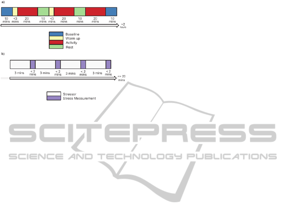
Figure 1: Session and activity structure. a) Session
structure. b) Activity structure.
Stressors: Our stressors included: Random
noises, cold water and a verbal mathematical test.
The control stressor (none) was simply having the
person perform the physical activity. The random
noises were composed mainly of sounds like: People
screaming, dogs barking and explosions. The math
test asked participants to subtract continuously from
a large number.
Baseline: During the baseline phase, the
participant relaxed and was asked to forgo any
posterior feelings and or thoughts. We used this as a
way to enforce stabilization of the physiological
signals.
Warm-up: In this phase, participant exertion was
increased by augmenting the speed of the physical
activity being performed, every 20 seconds until
reaching a predetermined speed. This speed, was
determined during the first session by asking the
subject to perform the given activity until his/her
heart rate level stabilized at about +/- 5% of 50% of
the maximal heart rate for walking and a minimum
of 60% of the maximal heart rate for bicycling. This
was done to ensure the safety of our participants,
minimize the risk of cardiac distress, and have
similar conditions across sessions and across
participants. Notice, however, that the maximal heart
rate of the participants is not the same; hence, the
speeds for each one were different. Despite this, the
exertion level according to their maximal heart rate
was similar. This phase lasted for 3 minutes.
The experimenter and the participant were the
only people in the room. Conversation between the
participant and the experimenter was kept to a
minimum. The order of the activities across the
study was determined using a counter-balanced
Latin square method. The inner structure of the
activities and general scheme did not change through
the whole experiment. For stress measurement, we
used a 5-point Likert scale (1 = calm state, 5 = most
stressful) to obtain subjective assessments of stress
by asking the participant. The scale was used
immediately after each activity and stressor pair was
administered. A total of 18 subjective stress levels
were collected, 12 from activities (3 activities times
4 stressors) and 6 after resting periods, warm ups
and the baselines.
4 DATA ANALYSIS
Our data set is composed of 336254 data points,
from a total of 20 different participants, from about
160 hours of data collection. From it, we discarded
the baseline data for the classification performance
tests. From the remaining data set, 49% of the data
had a reported stress level of 2 or higher (indicating
some stress). All of the data for participant 10,
session 3, and part of the data for participant 6,
session 4 was discarded due to malfunctioning of the
sensor system.
Before any pre-processing or classification, a
data analysis was performed. Different insights were
gathered through observation of the behavior of the
participant’s physiological signals during the
different phases of this study:
Participant’s physiological signals even during
a calm state do not have a small variance.
HR does not follow a unimodal distribution for
any of the activities.
Stressors impact on the physiological signals is
not visible.
In the next sections these insights are described.
4.1 Baseline
We believed that during the baseline, the participant
would return quickly to their most calm state
independent of previous activities. However, this
calm state did not have a small variance for half of
the participants across our study. One example of
this behavior can be seen in Figure 2a where we
have a participant with a relatively low variance in
what looks like a bimodal distribution for HR across
the study and another participant in Figure 2b with
what also looks like a bimodal distribution but with
a much higher variance for HR. The reasons for this
high variance are hard to attribute but given that the
highest variance was most often during the
participants’ last session, it is likely that it could
have been an effect of the season change.
PhyCS2014-InternationalConferenceonPhysiologicalComputingSystems
110
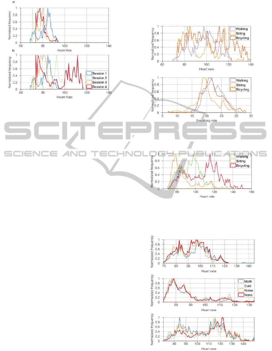
Figure 2: Histogram for the baseline heart rate for two
participants across different sessions. (a) Low variance
baseline for participant A. (b) High variance baseline for
participant B.
This high variance, however, was only observed
for the HR; the BR distribution had less variance and
was unimodal. The distributions for all the signals in
general can be summarized in the following manner:
HR is 55% unimodal and 45% multimodal, BR is
100% unimodal, GSR is 60% multimodal and 40%
unimodal, skin temperature is 100% multimodal.
The percentages refer to the quantity of all the
participant data; hence 100% represents all 20
participants.
4.2 Activities
To understand physical activity and its influence on
the physiological responses across the study,
histograms from all the physiological signals and
participants were obtained. One interesting pattern
found is shown in Figure 3, which corresponds to a
participant’s HR and BR during the entire study.
As expected the distribution of BR follows a
unimodal distribution, however, the same does not
hold true for HR, this was observed across all the
population. Also, it can be seen in Figure 4 that
across the entire population, HR had a multimodal
distribution. This means that there are not only
individual differences while performing the
activities across individuals, but also, the variance
within activities for each participant.
4.3 Stressors
In order to find out, in a descriptive way, whether
stress was expressed through the physiological
signals, we graphed the distribution of the HR for
the entire population throughout the study as can be
seen in Figure 5. A similar graph was produced also
for BR but the qualitative results were the same.
a)
b)
Figure 3: Histograms for Heart rate (a) and Breathing Rate
(b), from a single participant’s data across the four
sessions.
Figure 4: Heart rate histogram for all the population.
Variance across the different activities is so high that they
overlap each other making it harder to discern from single
values the activity performed.
Figure 5: Histogram for the heart rate of all the population
throughout the entire study for different activities. At the
top is the distribution for walking, middle for sitting and
bicycling is at the bottom.
StressRecognition-AStepOutsidetheLab
111
The distributions are quite similar, though there
are differences, which may be caused by random
errors from the measurement devices or from the
effects of the stressors. Still, this indicates that the
different stimuli used to exert stress did not play a
strong role in the variance of the physiological
signals. This finding shows that even in the absence
of physical activity, stressors do not visibly
influence physiological responses. Measurement of
the difference of the distributions by means of
correlation or other quantitative methods was not
conducted given the high visual resemblance among
the distributions.
5 PREPROCESSING AND
FEATURES
Next, we discuss how we pre-processed our data and
extracted features for the stress recognition task.
5.1 Labeling
For classification purposes the Likert scale values
were transformed to a binary class label: stress or
calm. The stress label corresponds to a Likert scale
of 2 or higher and the calm state corresponds to 1.
This means that our stress class covers from low
stress levels to high stress levels, while the calm
state covers only no stress. The labels were assigned
for the activity stressor pair. This means that if the
participant reported a Likert scale level of 3, for the
walking activity while the noise stressor was
administered, then all the data recorded during that
time was labeled as stress.
5.2 Preprocessing
The Bioharness is a high quality and recognized
commercial physiological signals recorder, however
for the HR measurement, this device relies on a
conductive fabric to be in contact with the
participant’s skin and on the participant to be
perspiring to acquire a high quality signal. The
conductive fabric pad of the Bioharness can slide
over the skin causing erroneous measurements to be
recorded or the signal to be lost for a short period of
time. This problem was minimized by asking the
participants to wear the band as tight as possible
without causing discomfort, but even after this
precaution, there was noise in the ECG signal caused
by sudden movements of the participants and initial
low perspiration levels. To address this problem, a
noise classifier was implemented and samples
classified as noise removed. For this task, different
algorithms were tried: Hidden Markov Models,
Naïve Bayes, Support vector machines and Logistic
regression using a ridge penalization. The models
were evaluated using a 10-fold cross validation test
and manually labeled data composed of 24 hours of
clean signals and 2 hours of noise from 6 different
subjects and 18 different sessions. The best noise
classifier was logistic regression and with 96%
accuracy.
5.3 Features
Research has shown that features based on the QRS
signal do a good job in affect recognition, but they
require costly and bulky sensor devices to get a good
quality signal. For that reason, in our work QRS
derived features were excluded and all of the
physiological signals came from a Zephyr
Bioharness and a Bodymedia Armband.
Preprocessing and extraction of further features was
limited to those approaches requiring low memory
and computing. The set of features can be seen in
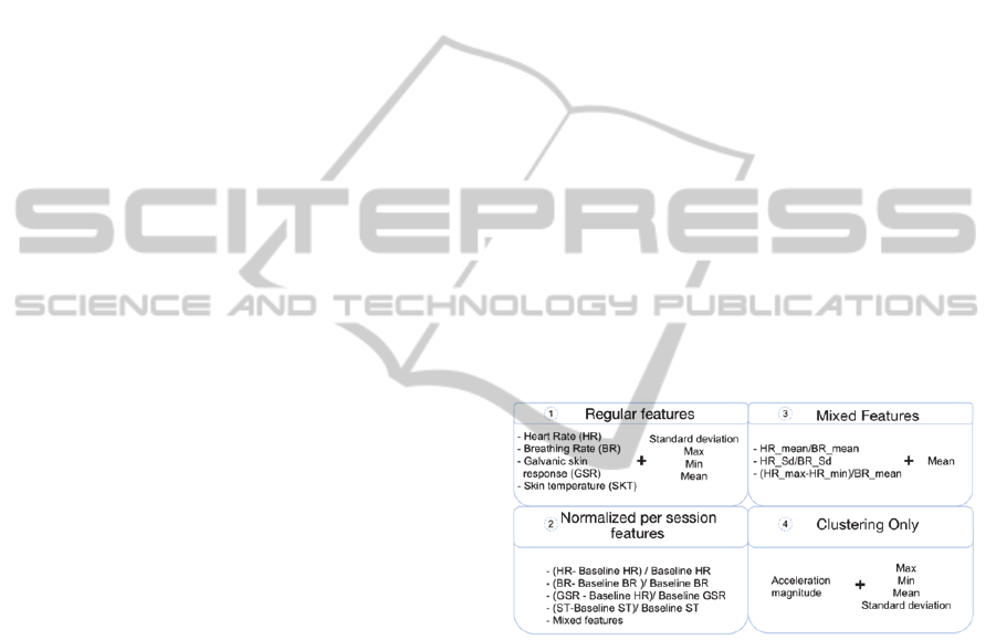
Figure 6.
Figure 6: Sets of features used.
A basic feature, namely a physiological signal
recorded by the Bioharness or the ArmBand, was
preprocessed by extracting simple statistics with
window sizes of 5, 10, 30 and 60 seconds. The
statistics used were: Mean, Maximum, Minimum
and the Standard deviation. The first set of features
called regular features is composed from basic
features and subsequent extraction of a particular
statistic. Feature set number two was created to
counteract variance across sessions by normalizing
each feature using the baseline data from that
session. These features were called the normalized –
per session features. For the third set of additional
features, the objective was to measure the
divergence between BR and HR. last, set number 4
shows the acceleration-based features, which were
used only for clustering.
PhyCS2014-InternationalConferenceonPhysiologicalComputingSystems
112
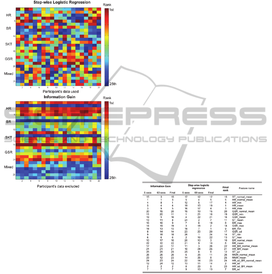
5.4 Feature Selection
Figure 7: Feature selection results. Features are listed on
the left of the heat maps, there are five different groups of
five features and the mixed features presented earlier.
Among the individual groups the features are organized in
the next manner: mean; standard deviation; max; min and
normalized per session feature. For the group of mixed
features the order is HR_mean/BR_mean then its
normalized version, HR_Sd/BR_Sd followed by its
normalized and last the (HR_max – HR_min)/BR_mean
and its normalized version.
In order to find out how many of the features
proposed significantly contributed to the stress
recognition task, we performed feature selection.
This was done using two different methods. In the
first, a leave-one-out cross-validation scheme
(Bishop, 2006) was used in conjunction with
information gain (Mitchell, 1997); the data for all
but one of the participants was used for evaluating.
Information gain was chosen because it is fast to
execute compared with other methods. The second
scheme used was greedy stepwise logistic
regression; for this, the data from every participant
was evaluated separately. Here, we wanted to find
out if there were features that would be the best for
all the participants while evaluating them
individually.
Results for a window of 5 seconds for
information gain and logistic regression can be seen
in Figure 7. We conclude that for scheme number
one, the effect on the population of removing one
participant's data was not significant. For scheme
number two, there is no visual pattern. This means
that there is not a single best set of features that
work for all people; instead there are subsets of
features that are good for some of the participants.
While the conclusions may seem contradictory, they
are, in fact, supportive of each other. Despite there
not being a single feature that is good across the
entire population, there are features that, on average,
have a high value for the stress recognition task.
Using the information from these two
experiments, we ranked the features, as shown in
Table I. The results show that all the features are in
general good, meaning there are not terrible features
that should be discarded. For example, the worst
feature had about half the ranking score of the best
feature.
Table 1: Features Ranking, The numbers denote the feature
while its position on the table denotes the rank. The final
rank is an average score created using the scores generated
for each of the single feature rankings from the information
gain and step-wise logistic regression.
6 STRESS RECOGNITION
In this section we explain the two steps used for the
training and testing of our stress recognition models.
Our method is a middle ground between
classification using a population model and
personalized models. This scheme separates the
population data according to their similarity into
subsets and for each of the subsets generated, creates
a stress model. The key difference between this
StressRecognition-AStepOutsidetheLab
113

approach and previous research is that we do not
cluster based on activity labels, which are likely not
to be available in real-world settings.
The recognition task is performed in a similar
fashion: First, the incoming data is recognized as
being part of one of the found subsets; then, the
corresponding stress model is used to perform the
stress recognition (see Figure 8). We used clustering
to find the subsets, and Naïve Bayes and Logistic
Regression to perform the stress recognition task.
All of our experiments were performed using Weka
(Mark et al., 2009) from within Matlab. For
clustering was used the Matlab K-means function,
for classification, we used the Naïve Bayes function
from Matlab and Logistic regression from Weka.
Figure 8: General structure of the clustering and
classification process. For training this scheme shows how
the data is used for creating the models. For testing, this
scheme shows how the data is clustered and used.
6.1 Clustering
Physical activity classification has shown good
results in the stress recognition task (Hong et al.,
2012). However, the human labels given to each of
the data points may not be the best descriptors of the
activities, or may not be available in real-world
settings given the huge number of activities that
people perform, nor are they the best way to separate
the data. During our data analysis, we concluded that
despite the measures taken to control the exertion
level, the HR was not following a unimodal
distribution within activities. This may be an
indicator of varying physical activity exertion level,
but it may also be a consequence of the stressor
administered during the activity. Independent of the
cause, this means there is a varying effort for the
heart to execute the activity. Hence, separating our
data based on activity, in order to create better stress
recognition models will not work since this
variability is not taken into account. Instead, if the
data is separated into low and high activity/exertion
levels, we accomplish the goal of dividing the data
according to the physiological signals’ behavior,
which in this case corresponds to separating the data
according to its quantitative properties. By
performing this separation, as we will see in the
results section, the stress recognition models
improve their performance.
Separating the data into low and high activity
levels is difficult; there are no labels from our
experiments or a clear way to measure the levels.
However, making use of K-means, we were able to
obtain a good separation of the data set. There are
many good clustering algorithms, but very often
many of them rely on an affinity matrix like
hierarchical clustering (Friedman et al., 2009) or
spectral methods (Ng et al., 2001), yet those
methods are not usable with our data set as their
memory use makes them prohibitive to run on a
single personal computer and the computation time
can last up to months. There exist methods to
approximate this affinity matrix, among them the
Nÿstrom approximation (Yan et al., 2009; Fowlkes
et al., 2004), however, for this data set, it did not
produce good results. These difficulties limited our
clustering methods to K-means. In our case we made
use of the K-means++ (Arthur and Vassilvitskii,
2007) algorithm that tries to maximize the distance
between the initial centroids of the desired clusters,
leading to better clusters in the exploration part of
K-means. Although limited to use K-means, the
results obtained show clusters that clearly separate
from high and low exertion levels. An example of
the average distribution of data among 2 clusters,
found by K-means for a 5-second can be seen in
Figure 9. The distribution of data for the 60-seconds
window is very similar to that shown in Figure 9.
This graph was created by averaging the cluster
contents from a 20-fold leave-one subject-out cross-
validation. The data set left out for testing
corresponds to a participant’s complete data set. To
determine the equivalence between the different
clusters found across the folds, we used the
correlation of the clusters’ contents.
Based on the correlation, the clusters were
grouped in two sets, and the average contents for
each set were calculated. Looking at the distribution
of data inside the clusters, we can see how the data
was divided into one cluster composed mainly of
bicycling and walking (i.e., high level of activity),
and another which contained walking, bicycling and
almost all the sitting, resting and baseline data (i.e.,
low level of activity).
PhyCS2014-InternationalConferenceonPhysiologicalComputingSystems
114
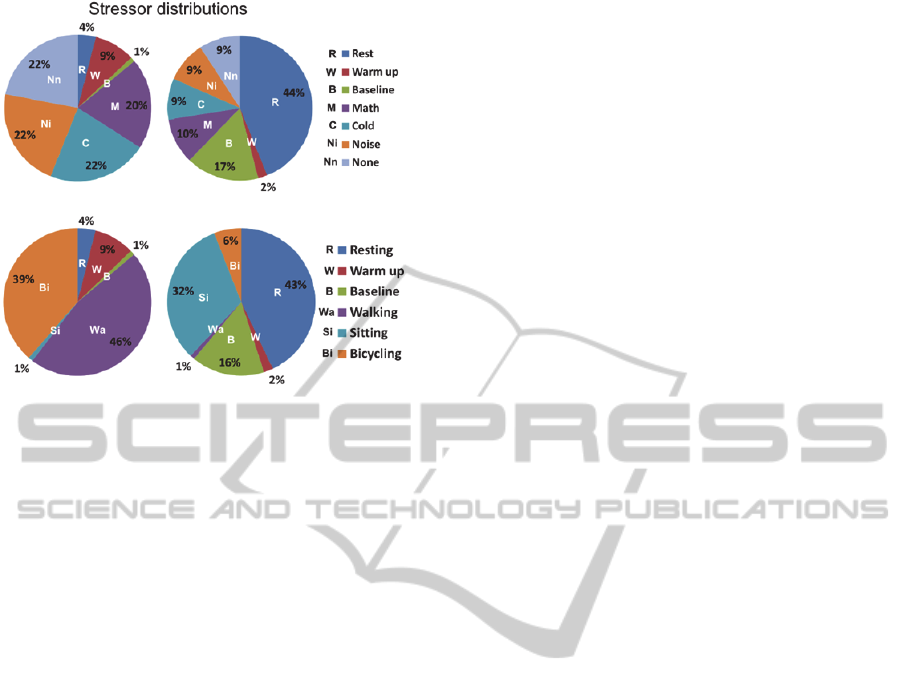
Figure 9: Average data distributions for two clusters and a
5 seconds window. Clusters on the left correspond to high
exertion level. On top: Average distribution for the two
clusters found and different stressors; looking at the
distribution, we can see the even allocation among
stressors indicating that these did not play a strong role in
the clustering. Bottom: Average distribution for the two
clusters found and different activities.
This natural separation of the data created by K-
means confirms our hypothesis that a better
separation of the data is achievable by using
clustering instead of classification. More
experiments were performed using a higher number
of clusters, however, for those the meaning of the
clustering becomes harder to interpret. Moreover,
there was no significant improvement in the
classification rate of stress by increasing the number
of clusters, making the additional computational and
memory burden unjustified.
6.2 Classification
For stress classification, Logistic regression was the
first model considered, since BR and HR are
correlated (they both increase while exercising) we
used the Ridge Penalization. The second model used
was Naive Bayes. In theory, this model does not
work with dependent features, however in practice it
has been shown to do a good job. The data used to
train the classification models is the data from the
clusters found by K-means.
6.3 Results
In order to measure the performance of the models
we used leave one out cross validation, where the
data set left aside comes entirely from one of the
participants. We had a total of 20 different
classification models and each was tested using
entirely unseen data by the models tested.
As a classification baseline, we used the scores
obtained from performing classification directly on
the data set without pre-clustering the data set. To
obtain the scores, the same cross-validation used
with the clustering + classification scheme was used
again. Results for classification only, show that the
classifiers do a good job in recognizing the calm
state (up to 0.76 f-measure), but their performance is
poor in recognizing stress (at best 0.29 f-measure).
A summary of the best results from the different
window sizes (5, 10, 30 and 60 seconds) can be seen
in Figure 10.
Our clustering and classification models were
tested using varying window sizes and different sets
of features: the window sizes used were: 5, 10, 30
and 60 seconds; the sets of features used for
classification are comprised of all-features (all) and
normalized-features (N); all-features are the regular
features, mixed features and normalized features.
For clustering, we used either all-features or only the
acceleration (Accel). By using only acceleration, we
were trying to see whether acceleration data was
sufficient to accomplish the clustering task. All the
data was standardized using the statistics from the
entire training data set, the same statistics that were
later used to standardize the testing data set. As a
performance metric in this work, we used accuracy
and the f-measure for each class: stress and calm
state. The reason for using the f-measure is to
overcome any imbalance in the ratio of the stress
and calm state data, caused by the clustering step.
This imbalance can cause accuracy to be an
overoptimistic measurement or completely
misleading as it could be indicating only the
performance of the classifier for recognizing the
biggest class. A total of 128 experiments were
performed using: 2, 3, 4 and 5 clusters; 5, 10, 30 and
60 seconds windows; 4 different sets of features
(classification used sets 1,2 and 3, clustering used 1,
2, and 3 as a single set and 4); two classification
algorithms Logistic regression and Naïve Bayes.
However, here we only report the results for the
extremes of the experiments, which summarize the
conclusions that can be derived from these
experiments. Results for logistic regression and two
clusters (Figure 12) for stress and a window of 5
seconds vary from 0.63 to 0.68 f-measure, across the
different sets of features. For a 60-second window
the f-measure varies from 0.6 to 0.68 (Figure 11).
The results for logistic regression and 5 clusters
have similar results as the 2 clusters model.
StressRecognition-AStepOutsidetheLab
115
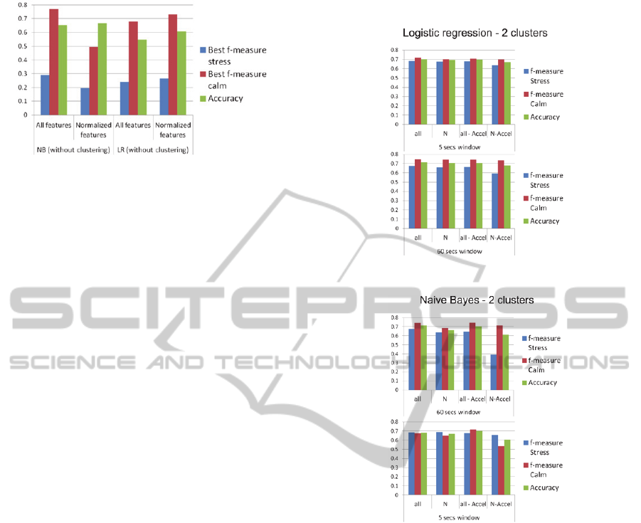
Figure 10: Baseline results for Logistic Regression and
Naïve Bayes without clustering.
The f-measure results for Naïve Bayes for two
clusters and 5 seconds (Figure 12) vary between
0.65 and 0.69. For the 60 second window, it varies
between 0.4 and 0.68 (Figure 12). For 5 clusters and
a 5 second window, the f-measure varies between
0.65 and 0.69. For 5 clusters and a 60 second
window, the f-measure varies between 0.42 and
0.62. All of the cluster-based results for f-measure
for stress (Figures 11 and 12) outperform the models
generated without clustering (Figure 10).
7 DISCUSSION
State of the art stress recognition systems have
shown accuracies of up to 90% (Ertin et al. 2011;
Plarre et al. n.d.) and emotion recognition systems
have shown accuracies ranging from 71.6% to
96.59% (Picard and Vyzas, 2001; Kim and André,
2008; Wagner et al., 2005; Kim et al., 2004;
Rainville et al., 2006; Lisetti, 2004). However, these
systems rely on very controlled settings and often
cannot work outside the lab. With respect to stress
with physical activity, none of the systems other
than our own previous work addresses this problem.
At best, one of these systems avoids measuring
stress when physical activity is detected (Plarre et
al., n.d.).
Our baseline comparison, which used Naïve
Bayes and Logistic regression, ignoring the activity
context, produces at most 65% accuracy. Our
previous work (Hong et al., 2012) which is the only
work tackling the problem of stress recognition
while performing a physical activity obtained an
accuracy of 87%. However, it relied on a set of three
activity labels which makes it impractical to
implement for real life stress recognition. Also, in all
of the aforementioned systems accuracy is the
performance measure, which can be overoptimistic,
as can be seen for our baseline results in Figure 10.
For this reason, we have relied on the f-measure for
both the stress and the calm state instead.
Figure 11: Results for 2 clusters and Logistic regression.
Figure 12: Results for 2 clusters and Naïve Bayes.
The method presented in this paper is a middle
ground in between state of the art approaches or
ideal systems, including our own previous work
which relies on prior knowledge about the data
collection, and a crude baseline, which could be
either chance (49% in our data set), or the results
obtained from using a bare classifier as shown in
Figure 10. We expect our system to perform better
than other systems under real life conditions because
it overcomes the following problems:
- Laboratory defined activities are different from
field activities: We were limited to the activities that
the participants performed during the study
(walking-running, biking, and sitting). However,
these activities, while common, do not cover the
whole spectrum of activities outside the lab like:
commuting, carrying objects, sitting in different
positions and surfaces, considering the weather. To
consider these, the data collection efforts would
increase by a factor of 4 for just this small set of
PhyCS2014-InternationalConferenceonPhysiologicalComputingSystems
116

activities. In this work, we have presented a method
that models the natural distribution of the data and
creates stress models on top instead of relying on an
activity label.
- The activity label is not the best way to classify
the context of the user: Even having a perfect
activity classifier, there is a broken assumption: that
the activity is generating some given spectrum of
physiological responses or that the physiological
responses across an activity, is somehow stable or
unimodal. We observed this is not the case in our
data set, which was collected on an already
constrained and controlled environment. This
problem can be expected to arise very often on an
outside of the lab deployment.
- Idiosyncrasies make activity recognition even
more challenging: From our own experience (Hong
et al., 2012) and others on (Ravi et al., 2005) how
people really walk, sit, and in general perform
activities, occurs in very different ways. This causes
activity recognition models to perform poorly (46%-
75% accuracy) on unseen or new data. Therefore, it
is even more unrealistic to expect to have activity
labels and to expect them to perform well in a big
field deployment where it may not be feasible to
build personalized models.
The method presented here boosts the
classification rate for stress compared to using only
the classifiers without any clustering. Even in the
worst case scenario there is a 33% improvement in
the f-measure for stress. At best, our scheme can
achieve up to a 130% improvement in f-measure for
the stress recognition task.
Despite our effort on including physical activity
in our experiment, many challenges still remain. For
example, our data set was small. Also it only
contains people between 18 to 38 years old with
good BMIs, which constitute a fairly healthy
population. In fact, only 6.4% of this age group is
reported to have a poor health status as compared
with 18.5% reported for those 45 years and over
(Schiller et al., 2012). Food ingestion, digestion and
metabolism play an important role in the stress
recognition. In our case, participants were asked to
refrain from consuming food 3 hours before coming
to the study and drinks or food containing caffeine
one day before every session. It has been shown that
caffeine increases the blood pressure (France and
Ditto, 1992) and hence it has a direct effect on the
heart responses. Also caffeine accrues with the
negative impact of stress on the immune system
(Feldman et al., 2004) and general health status.
However, it remains as an open question and an
interesting challenge, to determine whether
recognition of stress is possible while eating and its
impact on the stress recognition task. Of course,
another important future goal is to finally move out
of the lab environment and deploy stress recognition
for usage by people in their daily lives
8 CONCLUSIONS AND FUTURE
WORK
In this work, we have designed and developed an
approach that is more realistic than any other
previous work. Our approach does not rely on
intrusive or costly sensors, works in the presence of
physical activity and does not require activity labels
to work.
REFERENCES
American College of Sports Medicine, 2009. ACSM’s
Guidelines for Exercise Testing and Prescription 8th
ed., Williams & Wilkins.
Arthur, D. & Vassilvitskii, S., 2007. k-means ++ : The
Advantages of Careful Seeding. In SODA ’07
Proceedings of the eighteenth annual ACM-SIAM
symposium on Discrete algorithms. New Orleans,
Louisiana: Society for Industrial and Applied
Mathematics, pp. 1027 – 1035.
Bishop, C., 2006. Pattern Recognition and Machine
Learning, Springer-Verlag New York, Inc.
Ertin, E. et al., 2011. AutoSense. In Proceedings of the 9th
ACM Conference on Embedded Networked Sensor
Systems - SenSys ’11. New York, New York, USA:
ACM Press, p. 274.
Feldman, P. J. et al., 2004. Psychological stress, appraisal,
emotion and Cardiovascular response in a public
speaking task. Psychology & Health, 19(3), pp.353–
368.
Fowlkes, C. et al., 2004. Spectral grouping using the
Nystrom method. Pattern Analysis and machine
intelligence, 26(2), pp.1–12.
France, C. & Ditto, B., 1992. Cardiovascular responses to
the combination of caffeine and mental arithmetic,
cold pressor, and static exercise stressors.
Psychophysiology, 29(3), pp.272–282.
Friedman, J., Hastie, T. & Tibshirani, R., 2009. The
elements of statistical learning 2nd ed., New york:
Springer.
Giakoumis, D., Tzovaras, D. & Hassapis, G., 2012.
Subject-dependent biosignal features for increased
accuracy in psychological stress detection.
International Journal of Human-Computer Studies.
Healey, J. a. & Picard, R.W., 2005. Detecting Stress
During Real-World Driving Tasks Using
Physiological Sensors. IEEE Transactions on
Intelligent Transportation Systems, 6(2), pp.156–166.
StressRecognition-AStepOutsidetheLab
117

Hernandez, J. & Morris, R., 2011. Call center stress
recognition with person-specific models. Affective
Computing and Intelligent.
Hong, J.-H., Ramos, J. & Dey, A., 2012. Understanding
Physiological Responses to Stressors during Physical
Activity. In Proceedings of the 14th international
conference on Ubiquitous computing.
Kim, J. & André, E., 2008. Emotion recognition based on
physiological changes in music listening. IEEE
transactions on pattern analysis and machine
intelligence, 30(12), pp.2067–83.
Kim, K. H., Bang, S.W. & Kim, S.R., 2004. Emotion
recognition system using short-term monitoring of
physiological signals. Medical & biological
engineering & computing, 42(3), pp.419–27.
Liao, W. et al., 2006. Toward a decision-theoretic
framework for affect recognition and user assistance.
International Journal of Human-Computer Studies,
64(9), pp.847–873.
Lisetti, C. L., 2004. Using Noninvasive Wearable
Computers to Recognize Human Emotions from
Physiological Signals. EURASIP Journal on Applied
Signal Processing, pp.1672–1687.
Mark, H. et al., 2009. The WEKA Data Mining Software:
An Update. SIGKDD Explorations, 11(1).
Mitchell, T., 1997. Machine Learning, McGraw-Hill, Inc.
Ng, A. Y., Jordan, M.I. & Yair, W., 2001. On spectral
clustering: Analysis and an algorithm. ADVANCES IN
NEURAL INFORMATION PROCESSING SYSTEMS.
Novak, D., Mihelj, M. & Ziherl, J., 2011.
Psychophysiological measurements in a
biocooperative feedback loop for upper extremity
rehabilitation. … and Rehabilitation …, 19(4), pp.400–
410.
Picard, R. & Vyzas, E., 2001. Toward machine emotional
intelligence: Analysis of affective physiological state.
and Machine Intelligence,, 23(10), pp.1175–1191.
Plarre, K. et al., Continuous inference of psychological
stress from sensory measurements collected in the
natural environment.
Rainville, P. et al., 2006. Basic emotions are associated
with distinct patterns of cardiorespiratory activity.
International journal of psychophysiology : official
journal of the International Organization of
Psychophysiology, 61(1), pp.5–18.
Ravi, N., Dandekar, N. & Mysore, P., 2005. Activity
recognition from accelerometer data. In Proceedings
of the Seventeenth Conference on Innovative
Applications of Artificial Intelligence(IAAI. pp. 1541–
1546.
Robergs, R. & Landwehr, R., 2002. The surprising history
of the “HRmax= 220-age” equation. Journal of
exercise physiology, 5(2).
Roth, D., Bachtler, S. & Fillingim, R., 1990. Acute
emotional and cardiovascular effects of stressful
mental work during aerobic exercise.
Psychophysiology.
Schiller, J. S. et al., 2012. Summary health statistics for
U.S. adults: National Health Interview Survey, 2010.
Vital and health statistics. Series 10, Data from the
National Health Survey, (252), pp.1–207.
Sharma, N. & Gedeon, T., 2012. Objective measures,
sensors and computational techniques for stress
recognition and classification: A survey. Computer
methods and programs in biomedicine, 108(3),
pp.1287–1301.
Stäger, M., Lukowicz, P. & Tröster, G., 2007. Power and
accuracy trade-offs in sound-based context recognition
systems. Pervasive and Mobile Computing, 3(3),
pp.300–327.
Wagner, J., Kim, J. & Andre, E., 2005. From
physiological signals to emotions implementing and
comparing selected methods for feature extraction and
classification. In Multimedia and Expo, 2005. ICME
2005. IEEE International Conference on. pp. pp.940–
943.
Webb, H. E. et al., 2008. Psychological stress during
exercise: cardiorespiratory and hormonal responses.
European journal of applied physiology, 104(6),
pp.973–81.
Yan, D., Huang, L. & Jordan, M. I., 2009. Fast
approximate spectral clustering. Proceedings of the
15th ACM SIGKDD international conference on
Knowledge discovery and data mining - KDD ’09,
p.907.
Yao, Y.-J. et al., 2008. Heart rate and respiration
responses to real traffic pattern flight. Applied
psychophysiology and biofeedback, 33(4), pp.203–9.
PhyCS2014-InternationalConferenceonPhysiologicalComputingSystems
118
