
Addressing Signals Asynchronicity during Psychophysiological
Inference
A Temporal Construction Method
François Courtemanche
1
, Aude Dufresne
2
, Elise L. LeMoyne
3
and Esma Aïmeur
1
1
Department of Computer Science, University of Montréal, Édouard-Montpetit blvd., Montréal, Canada
2
Department of Communication, University of Montréal, Édouard-Montpetit blvd., Montréal, Canada
3
Tech
Lab, HEC Montréal, Louis-Colin av., Montréal, Canada
Keywords: Affective Signal Processing, Temporal Construction, Psychophysiological Inference, Triangulation.
Abstract: Predicting the psychological state of the user using physiological measures is one of the main objectives of
physiological computing. While numerous works have addressed this task with great success, a large
number of challenges remain to be solved in order to develop recognition approaches that can precisely and
reliably feed human-computer interaction systems. This paper focuses on one of these challenges which is
the temporal asynchrony between different physiological signals within one recognition model. The paper
proposes a flexible and suitable method for feature extraction based on empirical optimisation of windows’
latency and duration. The approach is described within the theoretical framework of the
psychophysiological inference and its common implementation using machine learning. The method has
been experimentally validated (46 subjects) and results are presented. Empirically optimised values for the
extraction windows are provided.
1 INTRODUCTION
The idea of a link between patterns of physiological
activity and psychological states is commonly
attributed to the American psychologist William
James (1842-1910) (Ellsworth, 1994). He suggested
that a person’s perception of emotion stems from
physical sensations caused by a reaction to a
stimulus. In the early 1990s, computer scientists
broadened this idea to create a new field of
research : physiological computing (Allanson and
Fairclough, 2004). The goal of physiological
computing is to translate bioelectrical signals from
the human nervous system into computational data.
A wide range of applications in human-computer
interactions, from brain-computer interactions to
affective computing, require the recording and
processing of the user's nervous system activity.
This paper focuses on one subfield of
physiological computing that aims to connect
physiological measures with psychological states. At
a theoretical level, this process is based on the
psychophysiological inference (Cacioppo and
Tassinary, 1990), and can be defined as follows: let
ψ be the set of psychological constructs (e.g. arousal,
cognitive load) and Φ be the set of physiological
variables (e.g. heart rate, pupil dilation). Cacioppo et
al., 2007 now describe the psychophysiological
inference according to the following equation:
Ψ = f (Φ)
The relationship f could be declined in four ways: 1)
one-to-one: a psychological state linked in an
isomorphic manner to a physiological variable, 2)
one-to-many: a psychological state reflects various
physiological variables, 3) many-to-one: various
psychological states related to a single physiological
variable, or 4) many-to-many: multiple
psychological states linked to multiple physiological
variables. The regulation of emotions relies at once
upon the sympathetic and parasympathetic activity
of the autonomic nervous system, whose activity is
also integrated in the central nervous system. The
regulation of emotion thus requires physiological
adjustments stemming from multiple response
patterns (Kreibig, 2010). Hence, relationships 1 and
3 have little chance of being sufficiently specific to
produce a valid inference. In fact, the relationships 2
and 4 dominate the psychophysiology literature.
However, when taking into account the difficulties
119
Courtemanche F., Dufresne A., L. LeMoyne E. and Aimeur E..
Addressing Signals Asynchronicity during Psychophysiological Inference - A Temporal Construction Method.
DOI: 10.5220/0004726801190127
In Proceedings of the International Conference on Physiological Computing Systems (PhyCS-2014), pages 119-127
ISBN: 978-989-758-006-2
Copyright
c
2014 SCITEPRESS (Science and Technology Publications, Lda.)

associated with isolating the physiological effects of
multiple simultaneous psychological states, most
works in physiological computing bring forth the
third relationship (many-to-one).
Numerous works have implemented the
physiological inference using a machine learning
framework (Picard et al., 2001, Christie and
Friedman, 2004, Haag et al., 2004, Bamidis et al.,
2009, Chanel et al., 2009, Verhoef et al., 2009,
Kolodyazhniy et al., 2011). Despite interesting
results, reported prediction accuracy rates are still
below the level of other machine learning problems
and cannot feed large-scale real-world applications
(van den Broek et al., 2010a). In a recent series of
papers, van den Broek et al. proposed 11
prerequisites to strengthen the foundation of this
field, which they coined Affective Signal Processing
(ASP) (van den Broek et al., 2009). In this paper, we
specifically address one of these problems; temporal
construction (van den Broek et al., 2010b). We
propose a method to take into account the temporal
differences while integrating different physiological
signals in a recognition process.
The remainder of the paper is as follows. Section
two presents the general inference framework used
in this paper and in most ASP approaches. Section
three describes the temporal construction problem in
the context of the later framework and our approach
to address this problem. The experimental validation
is presented in Section four and a discussion and a
conclusion are in Section five.
2 INFERENCE FRAMEWORK
Most works using the psychophysiological inference
follow more or less the six steps pipeline
summarised in Figure 1. The main goal is to gather a
data set, in which data points have the form [ψ
1
, ψ
2
,
ψ
3
, …, Φ], in order to train a recognition model f.
At step 1, the physiological signals Φ
i
are
selected according to their relation to the
psychological construct ψ that is to be inferred. In
this paper, three recognition models have been
trained to test the temporal construction solution: ψ
1
= emotional valence, ψ
2
= emotional arousal and ψ
3
= cognitive load, and five physiological signals have
been selected: Φ
1
= electrodermal activity, Φ
2
=
pupil size, Φ
3
= respiration, Φ
4
=
electroencephalography, and Φ
5
= cardiovascular
activity.
The goal of the elicitation step is to allow
subjects to experience different levels of the inferred
construct. Elicitation methods can be categorised as
being endogenous (relying on voluntary expression)
or exogenous (using stimuli) (Cowie et al., 2011).
Figure 1: Psychophysiological inference pipeline.
Whatever the method, the objective it to capture
the ground truth (G
T
) - the real state of the construct
for the subject - as precisely as possible. On the
other hand, the expected elicitation represents the
value that is anticipated and that will be inserted as
targets in the training data set (i.e. Φ in a data point).
The elicitation error (E
E
) can then be defined as E
E
=
| G
T
– Φ|. Since G
T
is related to the experiential
dimension of the construct, a certain level of
elicitation error is inevitable. As E
E
can considerably
impair the training process by inducing fuzzy
targets, different methods are used to minimise it.
The feature extraction step consists in
transforming the raw physiological signals in a data
representation that will serve as inputs for the
training algorithms. The choice of representation can
have a significant influence on the training process
and it is recommended to use domain knowledge in
doing it (Guyon and Elisseeff, 2003). In the field of
affective signal processing (ASP), most researches
use a feature-based approach, popularised by the
work of Picard et al. (Picard et al., 2001). As
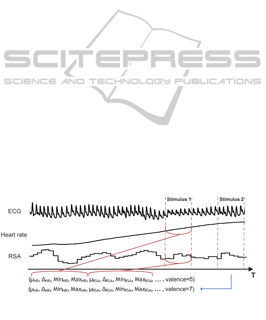
illustrated in Figure 2, this approach consists in three
main substeps. First, different underlying features
(e.g. Respiratory Sinus Arrhythmia (RSA), heart
rate) related to the inferred construct are derived
from the raw signal (e.g. Electrocardiogram - ECG).
The second substep consists in segmenting these
features according to the stimuli presentations.
During the last substep, different statistics are
calculated over each segment and for each feature
(e.g. average, standard deviation, min and max). The
latter statistics are the final ψ
i
attribute forming a
data point.
3 TEMPORAL CONSTRUCTION
Among the 11 prerequisites to improving the field of
PhyCS2014-InternationalConferenceonPhysiologicalComputingSystems
120
ASP presented by van den Broek et al. (van den
Broek et al., 2009), one of the most important is
temporal construction. More precisely, three main
problems are encountered concerning the temporal
aspects of physiological signals (van den Broek et
al., 2010b).
First of all, the habituation phenomenon implies
that the intensity of the physiological reactions to the
repeated presentation of a stimulus tapers off in
time. From the perspective of the
psychophysiological inference this means the
relationship Ψ = f (Φ) between a set of signals and a
psychological construct is not fixed in time. Other
elements must be considered in order to account for
the impact of previous occurrences of Ψ upon the
physiological reactions at a specific point in time.
The second problem concerns the law of initial
values. This law stipulates that “change of any
function of an organism due to a stimulus depends,
to a large degree, on the prestimulus level of that
function” (Wilder, 1958). The use of this law in
psychophysiology is subject to debate and it is
recommended to discuss the principle of initial
values instead (Jennings and Gianaros, 2007). While
this principle cannot be applied integrally and should
be nuanced, it remains that we can observe a
correlation between the prestimulus baseline of a
function and the direction and intensity of a reaction.
The final challenge concerning the temporality of
physiological activity is the asynchrony of signals.
As each physiological system operates in
collaboration with a variety of inputs and outputs
from the rest of the organism, the measured signals
present various durations and latencies for a given
stimulus. Heart rate for example may have a shorter
latency than Electrodermal Activity (EDA) for a
given stimulus. In this context, latency is defined as
the time elapsed between the presentation of a
stimulus and the beginning of a physiological
reaction. Duration is defined as the time elapsed
between the start and the end of a physiological
reaction. It is harder to identify the end of a reaction
as opposed to the beginning because the return to the
equilibrium of a signal is not necessarily equivalent
to the measured pre-stimulus baseline.
According to Gunes and Pantic, 2010, van der
Zwaag et al., 2010 and to the best of our knowledge,
the current literature on ASP offers no solutions to
these three temporal construction problems. We
were unable to find methodological approaches or
algorithms allowing for the process of inference to
take into account these temporal effects and to
improve the quality of recognition. Among the three
problems, we believe the most critical to be the
asynchrony of signals. First, because the
relationships 1 and 3 for the psychological inference
are not specific enough (see Section 1). Second,
because signal integration is at the heart of the
problem of triangulation of research tools in this
field. Asynchrony of signals is thus one of the main
obstacles in using multiple physiological signals
within a recognition approach. As can be seen in
Figure 2, the feature extraction step segments all the
signals at the same time point for a given stimulus.
The data vectors forming the training set therefore
contain attributes that do not optimally portray the
studied construct in regards to latency and duration.
3.1 Windows Optimisation
Our proposed solution for the problem of
asynchrony relies upon a flexible feature extraction
procedure, which allows modeling of the temporal
particularities of the various physiological measures.
The main idea is to optimise the latency and duration
of extraction windows. Furthermore, as suggested by
Figure 2: Feature extraction step.
AddressingSignalsAsynchronicityduringPsychophysiologicalInference-ATemporalConstructionMethod
121
van den Broek et al. (van den Broek et al.,
2010b),these two parameters should be optimised
according to the different constructs. Consequently,
an optimal extraction window should be determined
for each attribute and for each construct.
The identification of optimal latencies and
durations is done using an empirical optimisation
process. This optimisation was performed using the
data collected in the experiment described in Section
4. Let us take for example the optimisation of the
latency of the attribute µ EDA for the construct of
emotional arousal. Let n = the number of data points
in the training set and L = all possible latencies (e.g.
between 0 and 7000 ms, in increments of 100 ms).
For each latency L
i
, a table of size n x 2 is generated
containing n pairs [µ EDA, arousal] using an
extraction window with latency L
i
. A Pearson
correlation coefficient r
2
i
is then computed between
both columns of the table. The latency L
i
that
maximises r
2
i
will be selected as the optimal latency
for the feature extraction window of µ EDA for
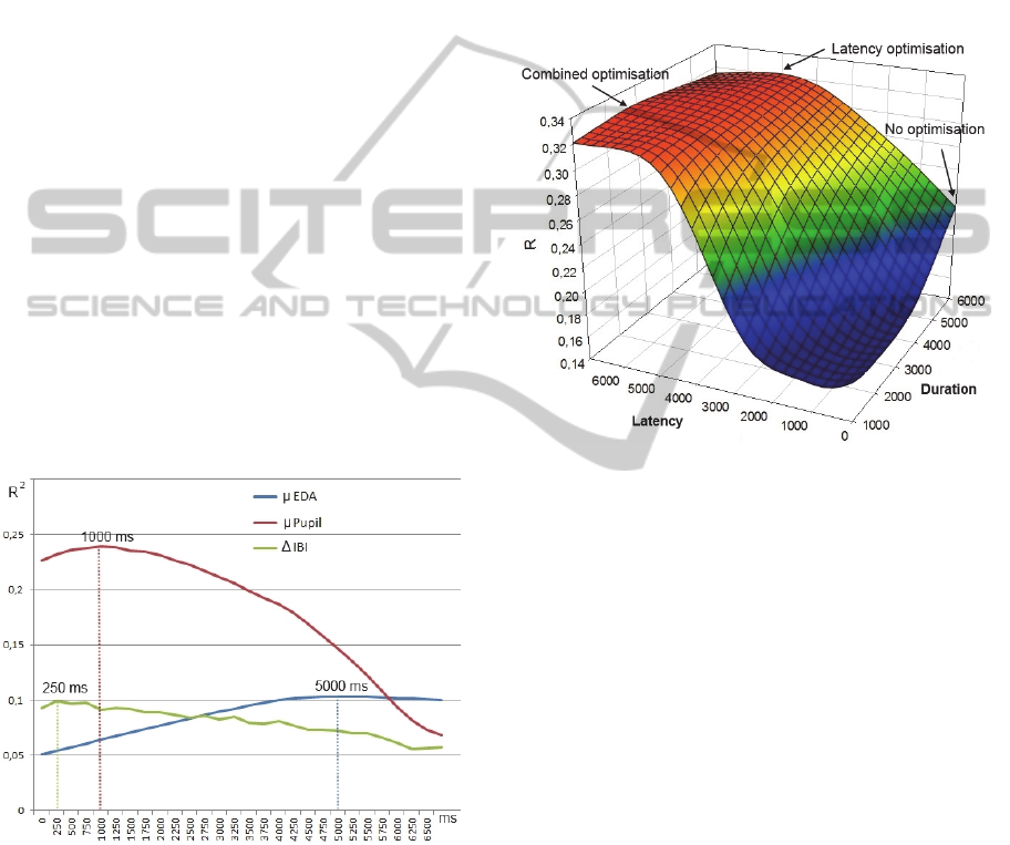
emotional arousal. Figure 3 illustrates various
latency values for three attributes (Δ interbeat
interval, µ EDA, and µ pupil size), for the construct
of emotional arousal. The latencies with the
maximal r
2
are identified with dotted lines (5000ms
for µ EDA, 250ms for Δ IBI (Interbeat Interval), and
1000ms for µ Pupil).
Figure 3: Empirical optimisation of windows latency.
In order to simultaneously optimise both
parameters of the extraction windows, the empirical
optimisation process is extended to include duration.
As illustrated in Figure 4 (for µ EDA), for each
latency L
i
and each duration D
j
, a Pearson
correlation coefficient r
ij
is computed.
The previously obtained optimal latency, 5000
ms, goes up to 7000 ms when jointly optimised with
duration for µ EDA. This shift on the optimisation
surface results in a slight increase of r of 0.01 (0.33
– 0.32). However, as opposed to the no optimisation
point (0, 6000) – stimuli were presented for 6
seconds (see Section 4.1.2) – the impact of the
combined optimisation of extraction windows
parameters upon r is more substantial (0.33 – 0.23 =
0.1). The average gain for the correlation
coefficients brought on by combined optimisation,
for all the attributes of the three inference models,
are of 0.08 (arousal), 0.06 (valence) and 0.14
(cognitive load).
Figure 4: Combined optimisation of latency and duration.
4 VALIDATION
This section presents the experimental validation
that was performed in order to assess the impact of
the optimisation of the feature extraction windows
on recognition performance.
4.1 Protocol
Fifty-two (52) participants (average age = 31) were
recruited for this experiment, an equal number of
men and women. A compensation of 40$ was
offered at the end of the session, which lasted about
1h30.
The physiological signals were collected at
250Hz using a Procomp Inifinity amplifier from
Thought Technology. Electrodermal activity (EDA)
was recorded at the phalange site. Cardiovascular
activity was recorded through blood volume
pressure (BVP) using a photopletismograph placed
on the middle finger. A respiration belt placed on the
upper chest was used to record respiration activity.
Electroencephalographic (EEG) activity was
PhyCS2014-InternationalConferenceonPhysiologicalComputingSystems
122
recorded using four electrodes on the F3, F4, P3 and
P4 sites following the 10-20 placement system.
These sites were selected in order to measure frontal
asymmetry (Coan and Allen, 2004). A 60 Hz notch
filter, and low-pass (1 Hz) and high-pass (60 Hz)
filter were applied to remove the electrical noise.
Finally, pupil size was measured using a Tobii X-120
eye-tracker. A simple normalisation procedure was
applied (x’ = x - µ
B
) using baseline data collected
during a two-minute resting period before
acquisition. For this work, 20 features were
extracted from the raw signals, for which 7 statistics
were calculated (mean, standard deviation, average
and absolute values of the first difference, min, max,
and kurtosis). Each data point in the training set is
initially composed of 140 attributes and one target.
4.1.1 Cognitive Load Elicitation
The first 15 participants did not complete the
cognitive load task. Amongst the 37 participants that
completed this part of the experiment, data from six
was rejected because of technical problems related
to the recording of physiological signals. Hence,
data from 31 participants was retained.
The protocol used to elicit cognitive load
consisted of an immediate serial recall task. Twenty-
four sequences of letters, varying between two and
seven letters, were presented to the participants.
They were asked to retain them for six seconds,
before repeating them out loud. The first 12
sequences were repeated in the same order they were
presented, while the following 12 were repeated in
the inverse order. The memorising was solely mental
and repeated voicing strategies were prohibited. The
presentation sequence of the stimuli is shown in
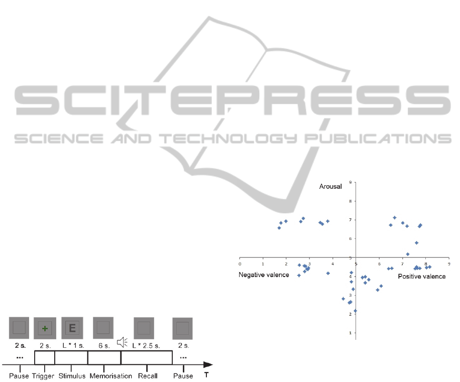
Figure 5.
Figure 5: Cognitive load stimuli presentation sequence.
The beginning of the sequence was indicated by
the presence of a green cross. Then followed the
sequence of letters, each presented for one second,
and the period of memorising. An audible beep
signaled when the presented sequence should be
repeated. This task provided 744 training examples.
4.1.2 Arousal and Valence Elicitation
Standardised stimuli composed of an image and a
related sound from the International Affective
Picture System (IAPS) (Lang et al., 2008) and the
International Affective Digitized Sounds (IADS)
(Bradley and Lang, 2007) collections were used to
elicit emotional arousal and valence. Forty-six
stimuli were presented for a period of six seconds
each. A bimodal stimuli approach was chosen in
order to confer a stronger ecological validity to the
elicitation (Anttonen and Surakka, 2005, Mühl and
Heylen, 2009). Self-evaluation using the SAM scale
(Bradley and Lang, 1994) has also been used in
order to reduce the elicitation error
(see Section 2).
All participants performed the affective stimuli
task. Data from eight of them were rejected because
of technical problems tied to the recording of
physiological signals. Hence, data from 44
participants was retained. While relying upon the
normalised evaluation of the valence and arousal of
the stimuli included in the IAPS, the images were
chosen in order to form five groups and uniformly
cover all quadrants of the emotional space. Figure 6
shows the distribution of the selected images.
Figure 6: Affective distribution of stimuli.
The distribution includes four non neutral groups
composed of eight images each: negative/low,
negative/high, positive/low and positive/high, as
well as a neutral group composed of 14 images:
neutral/very low. The sequence of the affective
stimuli presentations is depicted in Figure 7.
The general sequence, at the top of the figure,
alternates neutral and non-neutral block with a 20
second break in between each. The neutral and non-
neutral blocks respectively include two and four
stimuli. The bottom of the figure shows the sequence
of presentations within a block. It begins with a
AddressingSignalsAsynchronicityduringPsychophysiologicalInference-ATemporalConstructionMethod
123
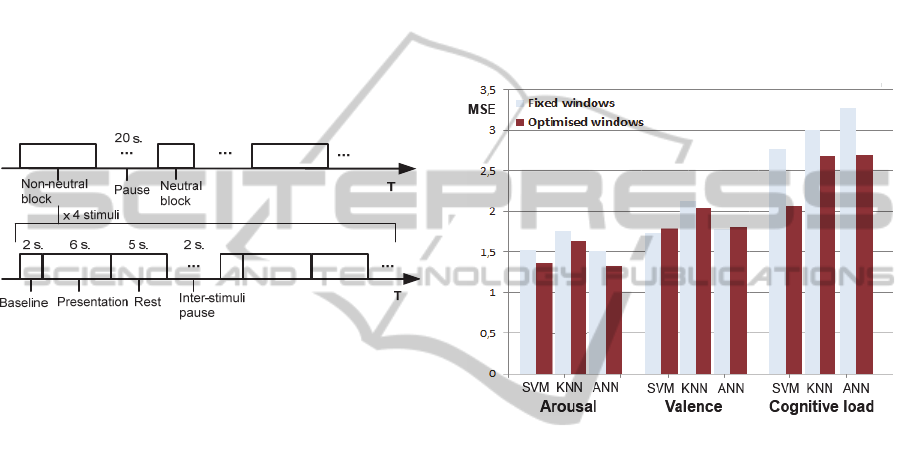
baseline (2 seconds), followed by the presentation of
a stimulus (6 seconds) and ends with a rest period (5
seconds). The presentation order of the non-neutral
blocks and the presentation order of the images
inside of the blocks are random. The images were
presented full screen and a green cross was
displayed for one second before each image. After
all 46 stimuli were presented, a self-assessment
interface was introduced showing all the previously
shown images in the same order. Underneath each
image were two scales based upon the Self-
Assessment Manikin (SAM) allowing for the rating
of the emotion felt at the time of the original
presentation. They were scored on a scale of 1 to 9.
This task produced 2024 training examples.
Figure 7: Affective stimuli presentation sequence.
4.2 Results
Prior to model training, a substep of feature selection
was performed in order to reduce the data
dimensionality and to keep only the more relevant
attributes. A variable ranking method based on
random probes was used (Guyon and Elisseeff,
2003), and 38 physiological attributes were selected
for the arousal model, 10 for the valence model and
51 for the cognitive load model. For emotional
arousal and valence, the targets are the average
between the subject's self-assessment and the
normalised values from the IAPS and IADS guides.
For the cognitive load model, the targets are the
number of letters to memorise (2 to 7). Since all
targets are numbers, the training of each model is a
regression problem. As we are interested in
assessing the impact of the proposed temporal
construction method on recognition performance
(and not recognition performance per se), three
different training algorithms were used: Support
Machine Vectors (SVM), k-Nearest Neighbor
(KNN) and Artificial Neural Networks (ANN). The
Statistica software from Statsoft was used to perform
training.
For machine learning regression problem, the
quality of the model's training is assessed using the
mean squared error (MSE), which is the average of
the squared difference between the predictions and
the actual values. Results are presented according to
this metric. Training of the SVM and KNN models
was executed following a k-fold cross validation
procedure with k=10. Training of the ANN model
was executed 10 times and the results averaged out
to account for the randomized elements involved in
the training procedure. In order to assess the impact
of temporal construction method upon the capacity
of the models to recognise the emotional/cognitive
state of a subject, the models were trained with and
without extraction windows optimisation. Results
are presented in Figure 8.
Figure 8: Impact of windows optimisation on MSE.
We can see that the mean squared error (MSE)
variation trends for each construct were consistent
amongst the different algorithms except for
emotional valence where two algorithms (SVM and
ANN) suffered a small error increase while one
algorithm decreased (KNN). The average variation
of MSE (over the three algorithms) for each model is
of -0.15 (arousal), 0.0 (valence) and -0.53 (cognitive
load). This results in average proportional gains for
the prediction performance of 9 % (arousal), 0 %
(valence) and 18 % (cognitive load).
5 DISCUSSION / CONCLUSIONS
van den Broek et al. proposed 11 prerequisites to
strengthen the foundation of affective signal
processing (van den Broek et al., 2009). This paper
presented a solution to the specific problem of signal
asynchrony. We demonstrated a method to
circumvent the temporal differences while
integrating many different signals in an
implementation of the psychophysiological
PhyCS2014-InternationalConferenceonPhysiologicalComputingSystems
124

inference Ψ = f (Φ). When the relationship f is used
on a one-to-many basis (a psychological state
reflects various physiological variables), the
elements of Φ react according to different temporal
scales (e.g. EDA at 4 seconds and ECG at 1 second
post stimulus). Until now, the feature extraction
methods used in the literature neglected this
phenomenon and segmented all signals according to
a stimulus using a single window.
Our temporal construction technique provides a
solution to the problem of signal asynchrony and
allows for a more optimal triangulation of multiple
signals and recording instruments by individually
optimising each extraction window for both latency
and duration. Results from this experiment showed
how the technique improved the quality of
recognition model of arousal by 9 % and of
cognitive load by 18 %. The valence recognition
model was not improved (0%) on the average and
reduced for two algorithms (SVM and ANN). A
possible explanation for this can be found in the
bipolar nature of the valence scale. As opposed to
arousal and cognitive load which increase in a
monotonous way, valence can be conceived as
evolving in two directions (positive or negative).
Indeed, it has been suggested to replace the bipolar
scale with two unipolar scales (van den Broek,
2011). With this in mind it is logical that a unique
relationship between values from the bipolar scale
and optimal temporal windows is hard to establish.
We now believe that different optimal windows can
exist for a given physiological signal, depending
upon the positivity or negativity of valence. Future
works should also include looking for gender, age or
personality effects on the value of the optimal
windows’ latency and duration. It could therefore be
possible to tailor more precisely the extraction
windows for specific subjects.
Following the large sample size of this study
(n=44 for valence and arousal and n=31 for
cognitive load), it can be expected that the
empirically optimised values for the extraction
windows can be used successfully in other studies.
To do so, we included in the Appendix (Figure 9)
the aforementioned values. Researchers working on
the physiological recognition of valence, arousal or
cognitive load could use these values while
segmenting signals according to their stimuli – being
that they are alike – and look for a gain in
recognition accuracy. The proposed approach could
also be adapted to different recognition contexts by
optimising extraction windows for various
physiological signals, psychological constructs or
stimuli.
ACKNOWLEDGEMENTS
This work was supported by NSERC (Natural
Sciences and Engineering Research Council of
Canada), the Canadian Space Agency and Bell
Canada. The authors would like to thank the Bell
Web Solutions User Experience Center for
providing the eye-tracker system used in this
research. We also wish to thank Laurence Dumont
for early comments on the manuscript.
REFERENCES
Allanson, J. & Fairclough, S. H. 2004. A research agenda
for physiological computing. Interacting with
Computers, 16, 857-878.
Anttonen, J. & Surakka, V. 2005. Emotions and heart rate
while sitting on a chair. SIGCHI conference on Human
factors in computing systems. Portland, Oregon, USA:
ACM.
Bamidis, P., Frantzidis, C., Konstantinidis, E., Luneski,
A., Lithari, C., Klados, M., Bratsas, C., Papadelis, C.
& Pappas, C. 2009. An Integrated Approach to
Emotion Recognition for Advanced Emotional
Intelligence. In: JACKO, J. (ed.) Human-Computer
Interaction. Ambient, Ubiquitous and Intelligent
Interaction. Springer Berlin / Heidelberg.
Bradley, M. M. & Lang, P. J. 1994. Measuring emotion:
The self-assessment manikin and the semantic
differential. Journal of Behavior Therapy and
Experimental Psychiatry, 25, 49-59.
Bradley, M. M. & Lang, P. J. 2007. The International
affective digitized sounds (2nd Edition; IADS-2):
Affective Ratings of Sounds and Instruction Manual.
Technical report B-3. University of Florida,
Gainesville, FI.
Cacioppo, J. T. & Tassinary, L. G. 1990. Inferring
psychological significance from physiological signals.
American Psychologist, 45, 16-28.
Cacioppo, J. T., Tassinary, L. T. & Berntson, G. 2007.
Handbook of Psychophysiology, New York:
Cambridge university Press.
Chanel, G., Kierkels, J. J. M., Soleymani, M. & Pun, T.
2009. Short-term emotion assessment in a recall
paradigm. International Journal of Human-Computer
Studies, 67, 607-627.
Christie, I. C. & Friedman, B. H. 2004. Autonomic
specificity of discrete emotion and dimensions of
affective space: a multivariate approach. International
Journal of Psychophysiology, 51, 143-153.
Coan, J. A. & Allen, J. J. B. 2004. Frontal EEG
asymmetry as a moderator and mediator of emotion.
Biological Psychology, 67, 7-50.
Cowie, R., Douglas-Cowie, E., Mcrorie, M., Sneddon, I.,
Devillers, L. & Amir, N. 2011. Issues in Data
Collection. In: COWIE, R., PELACHAUD, C. &
PETTA, P. (eds.) Emotion-Oriented Systems. Springer
AddressingSignalsAsynchronicityduringPsychophysiologicalInference-ATemporalConstructionMethod
125

Berlin Heidelberg.
Ellsworth, P. C. 1994. William James and emotion: Is a
century of fame worth a century of misunderstanding?
Psychological Review, 101, 222-229.
Gunes, H. & Pantic, M. 2010. Automatic Measurement of
Affect in Dimensional and Continuous Spaces: Why,
What, and How? In: SPINK, A. J., GRIECO, F.,
KRIPS, O. E., LOIJENS, L. W. S., NOLDUS, L. P. J.
J. & ZIMMERMAN, P. H. (eds.) 7th International
Conference on Methods and Techniques in Behavioral
Research, Measuring Behavior 2010. Eindhoven, the
Netherlands: Noldus.
Guyon, I. & Elisseeff, A. 2003. An introduction to
variable and feature selection. The Journal of Machine
Learning Research, 3, 1157-1182.
Haag, A., Goronzy, S., Schaich, P. & Williams, J. 2004.
Emotion Recognition Using Bio-sensors: First Steps
towards an Automatic System. In: ANDRÉ, E.,
DYBKJAE R, L., MINKER, W. & HEISTERKAMP,
P. (eds.) Affective dialogue systems. Springer Berlin /
Heidelberg.
Jennings, L. R. & Gianaros, P. J. 2007. Methodology. In:
CACIOPPO, J. T., TASSINARY, L. G. &
BERNSTON, G. G. (eds.) Handbook of
Psychophysiology. Third ed. New York: Cambride
University Press.
Kolodyazhniy, V., Kreibig, S. D., Gross, J. J., Roth, W. T.
& Wilhelm, F. H. 2011. An affective computing
approach to physiological emotion specificity: Toward
subject-independent and stimulus-independent
classification of film-induced emotions.
Psychophysiology, 48, 908-922.
Kreibig, S. D. 2010. Autonomic nervous system activity in
emotion: A review. Biological Psychology, 84, 394-
421.
Lang, P. J., Bradley, M. M. & Cuthbert, B. N. 2008.
International affective picture system (IAPS):
Affective ratings of pictures and instruction manual.
Technical report B-3. University of Florida,
Gainesville, FI.
Mühl, C. & Heylen, D. 2009. Cross-modal Elicitation of
Affective Experience. International Conference on
Affective Computing and Intelligent Interaction and
Workshops, ACII 2009, Workshop on Affective Brain-
Computer Interfaces. Amsterdam, The Netherlands.
Picard, R. W., Vyzas, E. & Healey, J. 2001. Toward
Machine Emotional Intelligence: Analysis of Affective
Physiological State. IEEE Transactions on Pattern
Analysis & Machine Intelligence, 23, 1175.
Van Den Broek, E. 2011. Ubiquitous emotion-aware
computing. Personal and Ubiquitous Computing, 1-
15.
Van Den Broek, E., Janssen, J., Westerink, J. & Healey, J.
Prerequisites for Affective Signal Processing (ASP).
In: ENCARNAÇÃO, P. & VELOSO, A., eds.
International Conference on Bio-inspired Systems and
Signal Processing, 2009 Porto, Portugal. INSTICC
Press, 426-433.
Van Den Broek, E., Janssen, J. H., Zwaag Van Der, M. D.
& Healey, J. A. Prerequisites for Affective Signal
Processing (ASP) - Part III. Third International
Conference on Bio-Inspired Systems and Signal
Processing, Biosignals 2010, 2010a Valencia, Spain.
Van Den Broek, E., Van Der Zwaag, M. D., Healey, J. A.,
Janssen, J. H. & Westerink, J. H. D. M. 2010b.
Prerequisites for Affective Signal Processing (ASP) -
Part IV. 1st International Workshop on Bio-inspired
Human-Machine Interfaces and Healthcare
Applications - B-Interface 2010. Valencia, Spain.
Van Der Zwaag, M. D., Van Den Broek, E. & Janssen, J.
H. Guidelines for biosignal driven HCI. ACM
CHI2010 workshop - Brain, Body, and Bytes:
Physiological user interaction, 2010 Atlanta, GA,
USA., 77-80.
Verhoef, T., Lisetti, C., Barreto, A., Ortega, F., Van Der
Zant, T. & Cnossen, F. 2009. Bio-sensing for
Emotional Characterization without Word Labels. In:
JACKO, J. (ed.) Human-Computer Interaction.
Ambient, Ubiquitous and Intelligent Interaction.
Springer Berlin / Heidelberg.
Wilder, J. 1958. Modern psychophysiology and the law of
initial value. American Journal of Psychotherapy, 12,
199-221.
PhyCS2014-InternationalConferenceonPhysiologicalComputingSystems
126

APPENDIX
LDLDLD LDLDLD
µ
0 1000 4750 1000 0 2600
µ
7000 6000 0 1000 0 1200
std 0 5750 0 1000 2200 1000 std 2750 4750 0 1000 3800 1000
µΔ 3000 1250 2750 2750 5800 3600 µ
Δ
0 1000 0 1000 0 1000
|Δ| 750 4250 0 1000 2200 1000 |Δ| 5000 1250 0 1000 3800 1000
min 1000 1250 3000 2750 0 1400 min 7000 6000 0 1000 200 1000
max 0 5750 6250 1250 7000 3600 max 7000 6000 0 1000 0 1200
kurtosis 4750 5500 3500 2500 2200 5800 kurtosis 6750 1750 0 2250 6200 1600
µ
7000 2250 0 1000 400 5600
µ
3000 6000 0 1000 0 1000
std 250 6000 6250 1250 2200 1000 std 4500 3000 1000 1000 0 1000
µΔ 4250 4750 5500 5500 2400 5400 µ
Δ
1000 1500 7000 3750 2800 5800
|Δ| 500 5750 0 1000 2200 1800 |Δ| 4500 2750 750 1000 0 1000
min 7000 1000 0 1000 4000 4600 min 3750 1250 0 1000 6800 1400
max 7000 4000 0 1000 1000 1600 max 2500 4750 0 1000 6000 5000
kurtosis 4750 5500 3500 2500 2200 5600 kurtosis 6750 3500 6500 6000 6000 4800
µ
0 1000 0 1000 5400 1600
µ
7000 2750 0 1000 7000 6000
std 2750 5750 0 1000 1800 1600 std 3500 2000 0 1000 7000 6000
µΔ 1000 2750 3750 2750 5000 1600 µ
Δ
3250 2000 6500 5500 6600 6000
|Δ| 5750 2000 0 1000 2000 1200 |Δ| 3750 1500 0 1000 6600 6000
min 0 1000 0 1000 5200 1000 min 7000 2250 0 1000 7000 4000
max 2750 5500 0 1000 3800 1400 max 5500 4250 0 1000 7000 6000
kurtosis 4250 5000 4000 3000 5800 4800 kurtosis 0 5000 0 1000 2400 1200
µ
0 1000 0 1000 0 1000
µ
0 1000 0 1000 0 1000
std 6250 2250 0 1000 0 1200 std 1000 1500 1500 1000 5400 3800
µΔ 6000 1250 7000 1750 0 1000 µ
Δ
3250 5750 3500 3500 5200 1000
|Δ| 6750 1500 0 1000 0 1200 |Δ| 1250 1500 0 2250 4400 5800
min 0 1000 0 1000 0 1000 min 0 1000 0 1000 0 1000
max 0 1000 0 1000 0 1000 max 7000 4750 1500 1000 6800 5800
kurtosis 0 1500 6750 1250 0 3800 kurtosis 2500 2250 5500 1250 1200 4200
µ
7000 6000 0 1000 0 1200
µ
500 1750 0 1000 0 1000
std 0 1000 0 1000 200 1000 std 0 1000 0 1000 3800 1000
µΔ 7000 2250 0 1000 0 1000 µ
Δ
0 3250 7000 2250 1400 1000
|Δ| 0 1250 0 1000 200 1200 |Δ| 5750 2000 0 1000 2000 1200
min 7000 6000 0 1000 0 1200 min 0 1000 0 1000 5200 1000
max 7000 6000 0 1000 0 1400 max 2750 5500 0 1000 3800 1400
kurtosis 0 1500 5750 4500 3400 1000 kurtosis 4250 5000 4000 3000 5800 4800
µ
3750 1000 0 1000 0 1000
µ
750 2250 0 1000 0 1000
std 0 1000 0 1000 0 1000 std 0 1250 7000 6000 3800 1000
µΔ 0 1000 0 1000 0 1000 µ
Δ
1000 3750 3500 5750 1400 1000
|Δ| 0 1000 0 1000 0 1000 |Δ| 1500 1000 0 1000 4000 2000
min 0 5250 0 1000 0 1000 min 750 2500 0 1000 0 1000
max 6000 6000 0 1000 0 1000 max 250 1500 0 1000 4600 4000
kurtosis 6250 1000 6500 1500 800 1200 kurtosis 2750 1750 4250 2750 0 2200
µ
7000 6000 0 1000 0 1200
µ
3750 1000 6500 1000 2000 6000
std 2750 4750 0 1000 3800 1000 std 7000 6000 0 1000 6600 5000
µΔ 0 1000 0 1000 0 1000 µ
Δ
1750 2500 2000 5250 0 2600
|Δ| 4250 2250 0 1000 2800 1000 |Δ| 6750 3750 0 1000 7000 5200
min 7000 6000 0 1000 0 1200 min 3250 1500 7000 2250 2600 1000
max 7000 6000 0 1000 0 1200 max 2250 2500 6500 1000 2200 2600
kurtosis 3250 1250 6500 1750 7000 2800 kurtosis 2500 1250 5500 1750 800 2200
µ
0 1000 7000 6000 7000 6000
µ
3000 1000 0 1000 0 1000
std 5750 3500 1000 1000 0 1000 std 750 1000 0 1000 1400 2000
µΔ 6500 1250 0 1000 0 1000 µ
Δ
0 1000 5750 1000 0 1000
|Δ| 5500 4250 1000 1000 0 1000 |Δ| 750 1000 750 1500 1600 1600
min 0 1000 3500 6000 7000 5000 min 1750 1750 0 1000 0 1000
max 0 1000 1000 1000 7000 6000 max 3500 1250 6500 5000 0 3200
kurtosis 1000 1750 3250 1250 1200 1200 kurtosis 2500 3500 6500 1500 5400 5200
µ
0 1000 0 1000 0 1000
µ
5500 3500 0 1000 0 1000
std 0 1000 4250 1250 0 1000 std 2750 1250 0 1000 7000 5000
µΔ 0 1000 0 1000 0 1000 µ
Δ
0 1000 1500 3250 2000 3600
|Δ| 0 1000 3750 2750 0 1000 |Δ| 2750 1000 0 1000 0 1000
min 0 1000 0 3000 0 1000 min 1500 3750 0 1000 0 1000
max 0 1000 0 1000 0 1000 max 5000 3000 0 1000 3000 1400
kurtosis 3750 2000 500 3500 4800 1000 kurtosis 2500 3500 6500 1500 4800 5600
µ
1500 6000 0 1000 0 5600
µ
4500 1000 7000 2000 7000 3200
std 7000 6000 0 1000 1600 4800 std 0 2000 7000 3750 4600 1400
µΔ 0 1000 0 1000 6800 1000 µ
Δ
500 1000 3000 4500 800 2800
|Δ| 7000 6000 0 1000 2000 3800 |Δ| 4750 2500 4750 1000 4000 1400
min 3000 1000 0 1000 1000 2400 min 4500 1000 7000 5500 7000 2400
max 7000 6000 0 1000 2400 1400 max 5000 1750 7000 1250 7000 5200
kurtosis 7000 6000 250 3250 400 1400 kurtosis 1500 5250 2750 6000 5000 6000
CL
Signal Feature Attribute
Arousal Valence
Attribute
Arousal Valence CL
Signal Feature
LF(%oftotal
power)
HF(average
power)
Resp.
Amplitude
LF/HF
(average
power)
(F3+P3)‐
(F4+P4)
HF(%oftotal
power)
VLF(%oftotal
power)
EEG
Amplitude
Skin
conductance
F3‐F4
P3‐P4
(F3+F4)‐
(P3+P4)
BVP
BVP
Respiration
rate
HRMax‐Min
LF/HF(%of
tota lpower)
VLF(average
power)
LF(average
power)
SizePupil
EDA
Heartrate
Interbeat
interval(IBI)
AddressingSignalsAsynchronicityduringPsychophysiologicalInference-ATemporalConstructionMethod
127
