
The Battle of the Giants
A Case Study of GPU vs FPGA Optimisation for Real-time Image Processing
Lars Struyf
1
, Stijn De Beugher
1
, Dong Hoon Van Uytsel
2
, Frans Kanters
3
and Toon Goedem
´
e
1
1
EAVISE, ESAT-PSI-VISICS, KU Leuven, Leuven, Belgium
2
eSATURNUS, Leuven, Belgium
3
InViso, Eindhoven, The Netherlands
Keywords:
Computer Vision, Real-time, GPU, FPGA.
Abstract:
This paper focuses on a thorough comparison of the two main hardware targets for real-time optimization of
a computer vision algorithm: GPU and FPGA. Based on a complex case study algorithm for threaded isle
detection, implementation on both hardware targets is compared in terms of resulting time performance, code
translation effort, hardware cost, power efficiency and integrateability. A real-life case study as described in
this paper is a very useful addition to discussions on a more theoretical level, going beyond artificial experi-
ments. In our experiments, we show the speed-up gained by porting our algorithm to FPGA using manually
written VHDL and to a heterogeneous GPU/CPU architecture with the OpenCL language. Also, issues and
problems occurring during the code porting are detailed.
1 INTRODUCTION
Many applications have high inherent parallelism
which can be exploited for substantial execution time
speed-ups. Especially for many image processing al-
gorithms, this is the case because of the straightfor-
ward data parallelism possibilities on pixel basis. At
the same time, execution speed is the heel of Achilles
of many vision applications, without real-time perfor-
mance they can not be practically applied in real life.
An example is the endoscopic image enhancement al-
gorithm we describe in this paper, which have to be
implemented with minimal latency in order not to im-
pede the surgeon’s hand-eye coordination during an
operation. Therefore, much effort is put in real-time
optimization of image processing algorithms.
The first step is always to perform machine-
independent optimisations on the algorithm. A good
example is the development of the SURF feature de-
tection method (Bay et al., 2008), as a faster alter-
native to SIFT (Lowe, 2004), by approximating the
filters used by block filters and exploiting tricks like
integral image pre-calculation.
If on a standard CPU-based platform the required
speed is not reached yet, a next obvious step is imple-
menting the algorithm on specific hardware, at which
the inherent parallelism can be exploited. This paper
focuses on two frequently used types of parallel hard-
ware, FPGAs and GPUs. FPGAs have shown very
high performance in spite of their low operational fre-
quency by fully extracting the parallelism. On the
other hand, recent GPUs support a large number of
cores, and have a potential for high performance in
many applications. However, the cores are grouped,
and data transfer between the groups is very limited.
Programming tools for FPGA and GPU have been de-
veloped, but the prevailing idea is that it is still diffi-
cult to achieve high performance on these platforms
with limited effort.
Both platforms have very distinct properties.
While GPUs excel in raw processing speed in terms
of operations per second, FPGAs are the summit of
flexibility. In this paper we port one complex image
processing algorithm to both platforms to be able to
compare the resulting time performance. Another im-
portant evaluation criterium will be the effort that is
needed for the code translation.
Relevant related work, also comparing GPU and
FPGA for image processing algorithms, include the
work of Cope et al. (Cope et al., 2005) and Asano
et al. (Asano et al., 2009), which were unfortunatly
limited to rather simple image processing tasks (color
correction and two-dimensional convolution filters),
and rather outdated. More recent work is that of da
Silva et al. (da Silva et al., 2013), which is targeted at
combining the power of GPUs with the flexibility of
112
Struyf L., De Beugher S., Van Uytsel D., Kanters F. and Goedemé T..
The Battle of the Giants - A Case Study of GPU vs FPGA Optimisation for Real-time Image Processing.
DOI: 10.5220/0004730301120119
In Proceedings of the 4th International Conference on Pervasive and Embedded Computing and Communication Systems (PECCS-2014), pages
112-119
ISBN: 978-989-758-000-0
Copyright
c
2014 SCITEPRESS (Science and Technology Publications, Lda.)

FPGAs in a hybrid FPGA/GPU platform. Their con-
clusions are that the usefullness of the combination is
limited, because of the confined data bandwith avail-
able between GPU and FPGA. However, in their pa-
per they also report on a comparison where the GPU
and the FPGA are used separately. Their results show
that the HLS FPGA compiler outperforms handwrit-
ten code and offers a performance comparable to the
GPU for the application studied.
The remainder of this paper is organised as fol-
lows. In section 2, the threaded isle detection al-
gorithm we start from is detailed. After that, our
code porting efforts towards both GPU (section 3) and
FPGA (section 4) are reported upon. Our results are
presented in section 5. We end with an evaluation in
section 6 and a conclusion in section 7.
2 ALGORITHM
2.1 Algorithm Overview
The goal of the algorithm studied in this paper is to vi-
sually highlight linear structures during videoscopic
inspections. An example result is included as Fig-
ure 1. The algorithm is a chain of four basic build-
ing blocks: preprocessing, feature detection, filtering,
and visualization.
2.1.1 Preprocessing
The image is reduced to a grayscale picture which
discrimates better between linear structures and the
surrounding areas. This step is highly application-
specific, but can be methodically optimized with su-
pervised training techniques, using a set of expert-
annotated images. In many cases a linear transforma-
tion of the RGB or HSV colorspace or a lookup table
will yield good results.
2.1.2 Feature Detection
The structures to be highlighted are linear. Hence,
any edge or ridge detector can be used to extract these
from the preprocessed image. The algorithm uses
oriented phase congruency energy features (Kovesi,
1999) which are able to detect both strong and weak
edges. This method is based on a convolution of the
image with a filter bank of 24 log-Gabor-filters, over
4 scales and 6 orientations. Other edge detecting fea-
tures such as canny gradient strength were found less
appropriate for our intended applications. Of course,
different features can be combined for other applica-
tions.
Figure 1: Vascularization highlighting algorithm illustra-
tion: (left) input image, (right) output image.
2.1.3 Filtering
The goal of the filtering step is to suppress the de-
tected lines that do not bear visual information with
respect to the application at hand. For instance, for the
vascularization highlighting application as described
in section 2.2, a region where a lot of short vessels go
in random directions is probably not pathologic and
therefore not interesting for the detection of tumors.
2.1.4 Visualization
In the last step the filtered mask is combined with the
original image. This step is probably the least inter-
esting from an image processing point of view, but
very important for the optimal transfer of the com-
puted visual information to the human end-user of the
application. For the vascularization highlighting ap-
plication, the saturation of the original image is glob-
ally reduced, while the filtered feature map obtained
in the previous step non-linearly modulates the satu-
ration locally.
2.2 Applications
Such a general linear structure detection algorithm is
useful in a broad range of applications. We detail a
few of them below.
The application that spurred the initial develop-
ment of the line detection algorithm discussed in this
paper is real-time vascularization highlighting dur-
ing endoscopic procedures. Preliminary experiments
have shown that this highlighting is very likely to en-
hance the human detection rate of pathologic tissue,
such as endometriosis and tumors. Most malignant
tumors are linked with increased vascularization and
unregular vessel patterns (Tyrrell et al., 2005), pre-
sumably because of a higher demand caused by ac-
celerated growth. The increased vascularization be-
comes visible around superficial tumors as a star-
shaped structure. While the tumor itself may be very
small and invisible, the vascularization pattern sur-
rounding it is a valuable visual guide towards it. The
TheBattleoftheGiants-ACaseStudyofGPUvsFPGAOptimisationforReal-timeImageProcessing
113

Figure 2: Images of cracks in polished marble acquired by
confocal laser microscopic photography.
same holds for endometriosis, which is also charac-
terized with increased angiogenesis, often to be rec-
ognized as parallel vessels.
Also in other disciplines like colonoscopy, bron-
choscopy, hysteroscopy, vascularizaton patterns are
important for the detection of intestinal, lung, and
uterine tumors.
The software implementation of a vasculariza-
tion highlighting application was already developed
by eSaturnus for early tests with a few key users.
This prototype can process 3 standard definition video
frames per second and per core of an Intel Xeon E3-
1200 CPU. The work on hardware-accelerated line
detection, as described in this paper, allowed this ap-
plication to deliver smooth, low-latency filtered video
on the same space and power footprint as the original
software-only implementation.
Besides medical applications also various indus-
trial applications benefit from real-time line detection.
One example is automatic crack detection in various
materials, such as natural stone (fig. 2), composites,
plastics, metals, glass and concrete. During produc-
tion or processing of these materials tiny cracks can
cause parts to break with high additional costs. Au-
tomatic detection of cracks in incoming raw materials
using a machine vision system before production can
be used to reduce these costs. Another application for
fast line detection is automatic alignment or placing
objects using robots.
2.3 Code Profiling
As a start, the more complex and time consuming
parts of the source code had to be identified. This
was done by profiling the code and analysing the re-
sult to detect the most time consuming parts. Since
the application uses images from a video stream as
input, some parts will be run for every frame, while
other parts are run only once. The profiling resulted
in one function comprising six time-consuming loops
through which were computed over every frame: the
six passes of different log-Gabor filters over the im-
age.
A second time-consuming part of the algorithm is
the preparation of the log-Gabor filter itself by com-
puting the coefficients. But because these filters are
kept fixed during the processing of a video stream
they can be precomputed and are not interesting to
spend optimisation effort on.
3 GPU OPTIMISATION
As explained above, we will implement this algorithm
on two different hardware platforms. This section will
detail our GPU implementation, while the next sec-
tion is about the FPGA implementation.
For the GPU implementation of this algorithm, we
chose for the OpenCL language, because of its ability
to target heterogeneous hardware platforms and its ex-
cellent code portability across different GPU vendors.
In the subsections below, we first give an overview of
OpenCL and its coding philosophy. After that, the
specifics of the code porting OpenCL we did are de-
tailed along with the best practices we learned from
this case. Timing results will be given in chapter 5.
3.1 OpenCL
Modern computer platforms include one or more
CPUs and GPUs (and even DSPs amongst others). All
these hardware types are designed and optimized for
a specific type of calculations. OpenCL, Open Com-
puting Language (Khronos, 2011), is a quite novel
open standard for heterogeneous computing. It is a
framework for writing programs that can use these
platforms in an heterogeneous way. This is in great
contrast to CUDA, developed by Nvidia, which can
exclusively used for Nvidea GPU hardware. OpenCL
allows to write an efficient and portable implementa-
tion of an algorithm which exploits the possibilities
for parallellizing parts of the algorithm on the most
suitable devices (multi-core CPU, GPU, celltype ar-
chitectures or other parallel processors). Since it is
heterogeneous, it is not nessecary to know in advance
which hardware will be used to execute the algorithm.
The used platform can easily be changed by changing
an initialisation variable of the program. Since differ-
ent devices have different instruction sets, the compi-
lation of the OpenCL kernels happens online (during
the execution of the program).
The code is written in the form of kernels. A ker-
nel is a block of code, written in a language based
PECCS2014-InternationalConferenceonPervasiveandEmbeddedComputingandCommunicationSystems
114
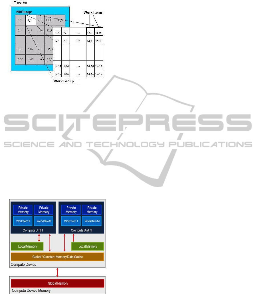
Figure 3: The execution of the kernels is divided in work-
groups, which can be subdivided in work items. Each work
item executes an instance of the kernel.
on C99, that can be executed in parallel. For exam-
ple, when each value of a matrix has to be multiplied
by a certain value, each kernel contains the code for
one multiplication and this kernel will be executed
for all elements of the matrix. The execution of the
NDRange (all kernels that have to be executed) is
subdivided into workgroups. A workgroup is subdi-
vided into work-items, which will execute the kernels
in parallel (figure 3). To distinguish between differ-
ent executing threads, each thread has a unique global
id, and within a workgroup each thread has a unique
local id. Both are assigned for each dimension.
Figure 4: Memory model of a GPU, from slow to fast:
Global memory, Local memory, Private memory.
Figure 4 shows the memory model of a GPU de-
vice. The memory access times are ranging from the
slowest at the bottom (starting with the memory of the
host computer) to the fastest at the top (private mem-
ory). The global memory of the GPU (and CPU) is
shared over all executing work items, the local mem-
ory is shared over the work items in the same compute
unit (workgroup) and the private memory is only ac-
cessible by the running work item.
3.2 Code Porting to OpenCL
OpenCL has the advantage that it is a middleware
built upon C/C++. Hence, porting an algorithm that is
already written in C/C++ to OpenCL is not that com-
plex.
The general approach was to identify the code that
had to be run for every image frame and search for
the loops within that code. Since OpenCL on GPUs is
highly parallel, embarrassingly enough, parallel loops
that iterate over every image pixel are the most effi-
cient to port to OpenCL for the biggest performance
gain.
Porting code to OpenCL can be divided in three
parts. First, the different loops must be ported to
OpenCL kernels, so they can be run on the GPU.
Since the code made use of the highly optimized Intel
Integrated Performance Primitives library, step 2 was
to find alternatives for these functions and also port
those to OpenCL. Included in this step is the merging
of several smaller loops into bigger ones. This way,
loops 2, 3 and 4 were merged into one, and the Intel
IPP functions were included in the loops most adja-
cent to them. Step 3 is the elimination of data traffic
between the host and the GPU, as this is very time
consuming over the slow PCI-Express bus.
We encountered some problems during this, al-
though most of them were quickly solved:
• The use of the Intel Integrated Performance Prim-
itives library took some time to get similar func-
tionality that could be ported to the GPU. Since
the IPP library makes excellent use of SSE in-
structions and multiple cores, it was sometimes
difficult to beat the performance of these func-
tions. Optimizing the OpenCL code was neces-
sary to getting higher performance on the GPU.
• Different DFT/iDFT libraries yield different re-
sults. Since the IPP library isn’t very well docu-
mented as to how the different functions are im-
plemented, switching to another library caused
some problems with the results. AMD has it’s
own OpenCL Math library, called APPML, which
can be used as an alternative for Intel’s IPP DFT
functions. But they too don’t share it’s implemen-
tation details with the user.
• Windows/Linux compatibility issues. These is-
sues can mostly be traced back to the different
implementation of the size_t type. In Windows,
this is always four bytes, as in OpenCL. In Linux,
on the other hand, it can be eight bytes for a 64-
TheBattleoftheGiants-ACaseStudyofGPUvsFPGAOptimisationforReal-timeImageProcessing
115

bit OS, the OpenCL size is still only four bytes
though.
The main lesson learned is that the simple tech-
nique of GPU-optimizing only the code parts that are
identified as the most computationally intensive by
the profiler is not a good idea. In many cases, little
is gained (or the result is even slower), because of the
increased need of CPU-GPU data traffic. Data local-
ity, i.e. keeping data as long as possible on the GPU,
is much more important.
3.3 Ease-of-use Evaluation of OpenCL
In this section we will discuss our experiences with
the use of OpenCL as a way to optimize an algorithm
by running it on GPU. We will comment on the learn-
ing curve and give tips and tricks for development.
Learning Curve. Since it is a quite novel standard,
the available literature is still growing. The spec-
ifications released by the Khronos group (Khronos,
2011) are very valuable as a reference for function
calls while developing. It does not only explain how
to use the functions, but also gives possible errors and
shows how to prevent them. Although it is a great
help, it does not contain enough information to ex-
ploit the possibilities of OpenCL to produce the best
implementation. It is necessary to know how OpenCL
works, to fully exploit these opportunities. When we
started using OpenCL, the learning was mostly based
on examples and a trial and error-approach, which re-
sults in a longer learning curve. Now, the available
literature (Tsuchiyama et al., 2009; Benedict et al.,
2011) offers a more complete range of books which
reduces the learning curve drastically and can also
teach the reader a correct way of programming for a
high performance gain.
Development. OpenCL focuses on heterogeneity.
This comes at the cost of a lot of function calls to
set up your execution environment (creating a plat-
form, creating devices, creating a program, creating
command queues, ...). This can be seen as a disad-
vantage, but once these functions are written, they
can easily be reused in later projects without losing
the flexibility it offers. This flexibility allows an easy
change of execution device without modifying your
kernel code. To make optimal use of the possibili-
ties of OpenCL, it is necessary to understand every
detail of the algorithm to implement. Just copy-and-
pasting existing source code to kernel code can give a
speed up, but this will be small compared to an imple-
mentation which exploits the availability of fast mem-
ory, the highest parallellization possible and sequen-
tial memory access. The upcoming amount of (pub-
lic) available libraries of optimized implementations
of commonly used functions (matrix multiplication,
image filtering, convolution, ...) can limit the devel-
oping time, since the developer only needs to focus
on the rest of the algorithm.
4 FPGA OPTIMISATION
4.1 Algorithm Adaptation
Since the architecture of an FPGA is completely dif-
ferent than the architecture of a GPU, not all algo-
rithms that can be ported successfully to a GPU can
also be successfully ported to an FPGA. If an algo-
rithm can be rewritten such that it can handle stream-
ing data without large memory blocks an FPGA im-
plementation is often possible. Examples of such al-
gorithms include simple image filtering operations,
where only a small neighborhood of pixels is neces-
sary at a certain moment. The first step in porting im-
age analysis algorithms into FPGAs is to rewrite the
algorithm into a streaming algorithm. In our research
first an attempt was made to convert the oriented
phase congruency energy features (Kovesi, 1999)
used by eSaturnus into a streaming algorithm that
fits the proposed FPGA (a Xilinx Spartan6 LX150).
The original algorithm uses 24 oriented log-Gabor
filters (4 scales, 6 orientations) which are not sepa-
rable in the spatial domain. Calculation in the fre-
quency domain however introduces the need for 24
parallel inverse Fourier transforms which do not fit
on the FPGA. An approximation in the spatial domain
using 3 separable Gaussian derivative kernels can be
made with good results (illustrated in fig. 5). This is
inspired by the DoG approximation of the Laplacian
(Mexican Hat function) in e.g. (Lowe, 2004). How-
ever, since 3 of these kernels are necessary for each
approximation for both the even and odd parts this
results in storing 144 separable filter results. With
relatively large spatial kernels (e.g. 21×21 pixels)
the internal memory of the FPGA for storage of the
line buffers is not sufficient on the targeted Spartan 6
FPGA. Not even the largest Virtex 7 FPGAs have the
required 2.880 BRAM blocks suitable for such imple-
mentations. Moreover, using external memory would
cost too much data transfer overhead. Therefore, we
switched to an alternative line enhancement algorithm
that yields similar results (in terms of PSNR) for the
FPGA implementation.
PECCS2014-InternationalConferenceonPervasiveandEmbeddedComputingandCommunicationSystems
116
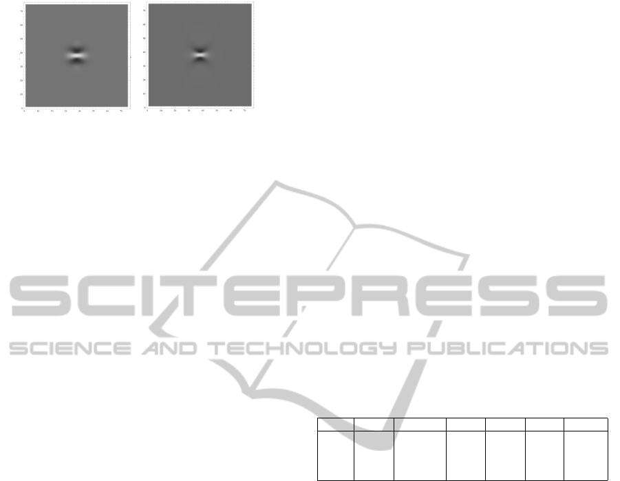
Figure 5: A log-Gabor filter (kernel shown on the left) is ap-
proximated by a combination of 3 Gaussian derivative ker-
nels (right).
4.2 Orientation Score Algorithm
The orientation score framework (Kalitzin et al.,
1999; Duits and Franken, 2010a; Duits and Franken,
2010b) has been proven very useful for line detec-
tion and enhancement. It is also based on a set of
oriented filters, similar to the log-Gabor filters used
in the phase congruency algorithm. However, instead
of calculating phase features in each pixel to enhance
lines a simple group convolution (a convolution not
only over the spatial domain, but also over the orien-
tation domain) is performed that is very suitable for
FPGA implementations. In our experiments 24 filters
are used (3 scales, 8 orientations) to have a compa-
rable complexity as the phase congruency algorithm.
The filters are not separable in the spatial domain and
are similar to the log-Gabor filters. The group convo-
lution is comparable in the number of multiplications
and additions to the phase congruency algorithm, but
can be better optimized for FPGA implementations.
4.3 FPGA Implementation
The orientation score algorithm is implemented di-
rectly in VHDL using simple arithmic operators, reg-
isters, multiplexers and FIFO (First In First Out)
buffers. The data is streamlined through a number
of registers and FIFO buffers in such a way that at a
certain clock cycle all necessary pixels for the N × N
neighborhood are present in registers. Then in parallel
the filter operations are performed resulting in all 24
filter results at a certain pixel position in each clock
cycle. These results are again streamlined through
a number of registers and FIFO buffers to obtain an
M × M × 24 neighborhood of all filter results to per-
form the group convolution, again resulting in one
value per pixel clock. This way, in each clock cycle
one pixel is loaded and one pixel result is presented.
The maximum clock frequency thus determines the
maximum amount of pixels per second that can be
processed. All calculations are fixed-point calcula-
tions with a flexible position of the point. This is pos-
sible without losing accuracy due to the carefully cho-
sen filter values.
5 RESULTS
In this section, we will first examine the timing re-
sults of the GPU implementation (5.1) and the FPGA
implementation (5.2) respectively.
5.1 GPU Results
First we will present the timing results of our
OpenCL-based GPU optimization. In table 1 the dif-
ferent steps of our GPU porting process, as described
in part 3.2, and their respective speed gains can be
found. Results are generated on an Intel Core i7 950,
6GB RAM, AMD Radeon HD6870 with Windows
7 Professional. The software used is Visual Studio
2010, with the AMD Accelerated Parallel Program-
ming (APP) SDK and AMD APPML (APP Math Li-
brary).
Table 1: GPU optimization: processing time/image (in ms)
for 720×576 resolution at different steps of the porting pro-
cess.
Loop 1 Loop 2,3,4 Loop 5 Loop 6 Total w/traffic
Ref. 122.0 214.78 7.14 52.28 396.21 408.40
Step 1 106.75 126.38 8.74 4.51 246.39 303.88
Step 2 67.45 5.24 0.071 5.66 78.54 166.18
Step 3 6.81 0.015 0.0026 0.0019 6.83 40.93
In the reference implementation and step 1 of the
port, loops 2, 3 and 4 were still separated from each
other in loops or different kernels. It is only in step
2 that these kernels were taken together to construct
one big OpenCL kernel. Doing this eliminated a lot
of data traffic from host to GPU and otherwise, which
accounts for the large gain in speed performance. In
step 3, the AMD library with FFT implementation in
OpenCL was used and all dependecies to the IPP li-
brary removed, what resulted in another tremendous
speed-up to 41 ms for a 720×576 image frame. Tak-
ing also the preprocessing and processing times in ac-
count, this boils dow to 65 ms, or more than 15 fps.
The resulting processing speed for different image
resolutions is given the graph of figure 6. We can see
that for smaller images of e.g. 360×288, the resulting
speed is even more impressive: about 14 ms or about
30 fps.
When reducing the number of scales or orienta-
tions filtered at, the framerate increases also. At 3
scales (instead of 4), SD video is processed at 18 fps.
When the number of orientations is reduced to 4 in-
stead of 6, the framerate is 24 fps.
TheBattleoftheGiants-ACaseStudyofGPUvsFPGAOptimisationforReal-timeImageProcessing
117
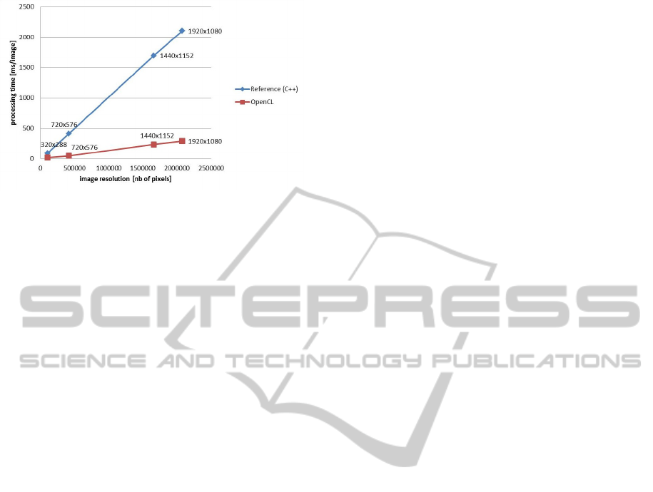
Figure 6: Processing speed results of the GPU implementa-
tion as compared to the reference C++ code started from.
5.2 FPGA Results
The VHDL code is synthesized using the Xilinx ISE
for a Spartan 6 LX150 FPGA. Using a gigabit Ether-
net connection the image data is loaded into the FPGA
and the results are sent back to the PC again. The Gi-
gabit Ethernet PHY (Physical layer) runs at 125MHz
with 8 bits in parallel. Since we use 8 bits per pixel
this results in a pixel clock of 125 Mega Pixel (MP)
per second. The VHDL design runs at 125MHz and
is thus also capable of processing the image at 125
MP per second. Before the output is valid however,
the FIFO buffers need to be filled. The delay between
first pixel in and first pixel out is in total a bit over
12000 clock cycles which results of a delay of 96 mi-
croseconds. In practice the demonstration unit is lim-
ited to the bandwidth of the gigabit Ethernet interface
which is below 125 MP per second due to overhead
of the packets. A Full HD video stream at 30 frames
per second is successfully tested.
6 EVALUATION
As explained above, we evaluated different criteria of
the two implementations: speed performance, code
translation effort, hardware cost, power efficiency, in-
tegrateability and physical space.
6.1 Speed Performance
On GPU, we achieved real-time performance on stan-
dard definition (SD) video (15 fps at 720×576 pix-
els). This is already quite impressive, compared to
our initial CPU implementation which only ran at 2
fps at that resolution. But the FPGA implementation
surpasses this greatly by showing timing results of 30
fps at HD resolution (1920×1080 pixels).
6.2 Code Translation Effort
While code porting to GPU via OpenCL was straight-
forward, an implementation on FPGA was much
more of a hassle. The only actual issue for
the OpenCL implementation was finding OpenCL-
versions of proprietary CPU-optimized software li-
braries. For the FPGA implementation, we were not
able to directly port the available algorithm. After
spending quite some time searching for approximated
filter kernels, this approach proved unfeasible. There-
fore, we had to make use of a totally different line
detection algorithm for the FPGA version. Moreover,
next to the tedious VHDL coding of the FPGA im-
plementation itself, we spent lots of effort to get the
CPU-FPGA interface working. Happily enough, both
FPGA and GPU developments took about 2-3 man
months because of the experiencedness of our FPGA
developer at InViso.
6.3 Hardware Cost
The actual hardware cost of the two platforms is com-
parable. The mainstream AMD GPU board that we
used in our demonstrator can be bought for around
e 160, while the Spartan 6 board is around e 200.
Note that the compared prices are for evaluation
boards only. The naked component cost for self-
assembly is also not significantly different.
6.4 Power Efficiency
When measuring the power usage of both platforms
(in full function) with a Watt meter, we observed that
the GPU consumed 65W extra on top of the 135W of
the PC itself, while the FPGA took less than 10W.
6.5 Integrateability
Although the impressive speed gain results of our
FPGA implementation, the integration of such a
hardware platform in an existing PC-based comput-
ing platform showed not obvious. We encoutered
quite some issues during interfacing between PC
and FPGA, which in the end was solved as a UPD
Ethernet connection. Moreover, we see that the
overall processing speed of the FPGA platform was
severely constrained by that interface. For GPU
hardware, these problems were non-existent because
of the seamless hardware integration and the fact
that OpenCL is developed for hybrid CPU/GPU plat-
forms.
PECCS2014-InternationalConferenceonPervasiveandEmbeddedComputingandCommunicationSystems
118

6.6 Physical Space
We see that the FPGA solution ended up very effi-
cient in terms of board space: the unit measures only
5cm×4cm. The computational density of the GPU
solutions is an order of magnitude worse, because the
AMD7850 is a PCB of about 26cm×12cm (with two
huge fans), which even does not fit in a standard desk-
top case.
7 CONCLUSIONS
In this paper, we have compared the optimal imple-
mentation of a complex image processing algorithm
on GPU and FPGA. On both target platforms, we
achieved an impressive speed-up factor, albeit with
quite different amounts of effort.
In general, we can conclude that both FPGA and
GPU platforms have important — but different — ad-
vantages. While the ultimate flexibility of a FPGA-
based system can lead to a speed performance that is
an order of magnitude better than the GPU-based plat-
form, the effort spent in developing a FPGA imple-
mentation of a certain algorithm boils down to quite
more effort as compared to the C/C++ to OpenCL-
translation needed for a GPU implementation. More-
over, we saw that the original algorithm was unsuited
to be implemented in a FPGA, even after an approx-
imated simplification, which forced us to rethink the
algorithm and move to a totally different approach. In
terms of physical space and power consumption, the
FPGA is certainly the winner.
Nevertheless, because of the ease to integrate the
GPU implementation in an existing server installa-
tion, eSaturnus chose the latter. At this moment, our
GPU code is running in a real hospital in Berlin as a
clinical try-out.
ACKNOWLEDGEMENTS
This work is partially supported by the European
Commision in the CrossRoads project of the Interreg
IVA program Border Region Flanders-Netherlands.
REFERENCES
Asano, S., Maruyama, T., and Yamaguchi, Y. (2009). Per-
formance comparison of fpga, gpu and cpu in image
processing. In International Conference on Field Pro-
grammable Logic and Applications (FPL), pages 126–
131.
Bay, H., Ess, A., Tuytelaars, T., and Gool, L. V. (2008).
Speeded-up robust features (surf). Computer Vision
and Image Understanding, 110.
Benedict, G. R., David, K., Perhaad, M., and Dana, S.
(2011). Heterogeneous Computing with OpenCL.
Morgan Kaupmann.
Cope, B., Cheung, P., Luk, W., and Witt, S. (2005). Have
gpus made fpgas redundant in the field of video pro-
cessing? In Proceedings of IEEE International Con-
ference on Field-Programmable Technology, pages
111–118.
da Silva, B., Braeken, A., D’Hollander, E., Touhafi, A.,
Cornelis, J., and Lemeire, J. (2013). Performance
and toolchain of a combined gpu/fpga desktop. In In
Proceedings of the ACM/SIGDA international sympo-
sium on Field programmable gate arrays (FPGA ’13),
pages 274–274, New York, NY, USA. ACM.
Duits, R. and Franken, E. M. (2010a). Left invariant
parabolic evolution equations on SE(2) and contour
enhancement via invertible orientation scores, part I:
Linear left-invariant diffusion equations on SE(2).
Quarterly of Applied mathematics, AMS, 68:255–292.
Duits, R. and Franken, E. M. (2010b). Left invariant
parabolic evolution equations on SE(2) and contour
enhancement via invertible orientation scores, part I:
Nonlinear left-invariant diffusion equations on invert-
ible orientation scores. Quarterly of Applied mathe-
matics, AMS, 68:293–331.
Kalitzin, S. N., Romeny, B. M. H., and Viergever, M. A.
(1999). Invertible apertured orientation filters in im-
age analysis. IJCV, 31:145–158.
Khronos (2011). OpenCL - the open standard for paral-
lel programming of heterogeneous systems. Khronos
Group.
Kovesi, P. (1999). Image features from phase congruency.
Videre: A Journal of Computer Vision Research, 1.
Lowe, D. (2004). Distinctive image features from scale in-
variant keypoints. International Journal on Computer
Vision, 60:91–110.
Tsuchiyama, R., Nakamura, T., Lizuka, T., Asahara, A.,
and Miki, S. (2009). The OpenCL Programming book.
Fixstars.
Tyrrell, J., Mahadevan, V., Tong, R., Brown, E., R.K., R. J.,
and Roysam, B. (2005). 2-d/3-d model-based method
to quantify the complexity of microvasculature im-
aged by in vivo multiphoton microscopy. Microvas-
cular Research, 70:165–178.
TheBattleoftheGiants-ACaseStudyofGPUvsFPGAOptimisationforReal-timeImageProcessing
119
