
Adaptation Schemes for Question's Level to be
Proposed by Intelligent Tutoring Systems
Rina Azoulay
1
, Esther David
2
, Dorit Hutzler
3
and Mireille Avigal
4
1
Department of Computer Science, Jerusalem College of Technology, Jerusalem 91160, Israel
2
Ashkelon Academic College, Ashkelon, 78211, Israel
3
Department of Computer Science, Jerusalem College of Technology, Jerusalem 91160, Israel
4
Computer Science Division, The Open University of Israel, Raanana, Israel
Keywords: Intelligent Tutoring Systems, Reinforcement Learning, Bayesian Inference.
Abstract: The main challenge in developing a good Intelligent Tutoring System (ITS) is suit the difficulty level of
questions and tasks to the current student's capabilities. According to state of the art, most ITS systems use
the Q-learning algorithm for this adaptation task. Our paper presents innovative results that compare the
performance of several methods, most of which have not been previously applied for ITS, to handle the
above challenge. In particular, to the best of our knowledge, this is the first attempt to apply the Bayesian
inference algorithm to question level matching in ITS. To identify the best adaptation scheme based on this
groundwork research, for the evaluation phase we used an artificial environment with simulated students.
The results were benchmarked with the optimal performance of the system, assuming the user model (abili-
ties) is completely known to the ITS. The results show that the best performing method ,in most of the envi-
ronments considered, is based on a Bayesian Inference, which achieved 90% or more of the optimal per-
formance .Our conclusion is that it may be worthwhile to integrate Bayesian inference based algorithms to
adapt questions to a student's level in ITS. Future work is required to apply these empirical results to envi-
ronments with real students.
1 INTRODUCTION
Intelligent Tutoring Systems (ITS) are based on
artificial intelligence methods (Woolf, 2009) to cus-
tomize instruction with respect to the student's capa-
bilities that dynamically change over the tutoring
period. To accomplish this, an ITS should contain
knowledge about the student's capabilities, termed
the student's model, and a set of pedagogical rules.
A critical characteristic of an ITS is the ability to
challenge students, without discouraging them due
to exaggerated challenges. Namely, on the one hand
the system should not provide questions to the stu-
dent that are too easy and leave him bored, while on
the other hand, the questions should not be too hard
to the point that they discourage the student from
using the system. In both of these extreme cases the
student will not realize its potential and therefore
will not benefit from using it. Therefore, we aimed
to construct an ITS that will match the hardest chal-
lenges the user can face and by doing so realize his
potential.
According to state of the art, most ITS systems make
use of the Q-learning algorithm for this adaptation
task. Our paper presents innovative results that com-
pare performances of several methods, most of
which have not been previously applied in ITS, to
handle this challenging adaptation task. In particu-
lar, to the best of our knowledge, this is the first
attempt to apply the Bayesian inference algorithm in
ITS for question level adaptation.
The leading principles involved in the develop-
ment of an efficient ITS include keeping track of
dynamically improving capabilities and knowledge,
and keeping the user active and satisfied. These are
achieved by considering the correctness of the an-
swers the student provides hitherto to the ITS. In
particular the ITS must choose a fixed number of
questions from a pre-prepared pull of questions to
present to the student. Obviously, the system is not
faced with a single decision for all the questions, but
instead question by question decisions, while taking
into account the history of the student's answers.
To enable a comparison between the various
245
Azoulay R., David E., Hutzler D. and Avigal M..
Adaptation Schemes for Question’s Level to be Proposed by Intelligent Tutoring Systems.
DOI: 10.5220/0004732402450255
In Proceedings of the 6th International Conference on Agents and Artificial Intelligence (ICAART-2014), pages 245-255
ISBN: 978-989-758-015-4
Copyright
c
2014 SCITEPRESS (Science and Technology Publications, Lda.)

proposed adaption schemes, we defined a utility
function to reflect the efficiency of each chosen
question. Specifically we considered the following
adapting schemes: (i) Q-learning (Sutton and Barto
2005, Rusell & Norvig 1995, Martin and Arroyo,
2004); (ii) Virtual Learning (Vreind, 1997); (iii)
Temporal Reasoning (Beck, Woolf and Beal 2000) ;
(iv) DVRL (Azoulay-Schwartz et al., 2013); (v)
Bayesian Inference (Conitzer and Garera, 2006); and
(vi) Gittins Based Method (Gittins, 1989). Most of
the algorithms have not been used for ITS, excluding
the Q-learning method which has been used for ITS,
as discussed in Section 2.
As this is a groundwork research to identify the
best adaptation scheme, at this stage of the study we
developed an artificial environment by simulating
students with ability distributions derived from a
normal distribution.
The performance of the various proposed meth-
ods were benchmarked with the optimal perfor-
mance of the system assuming the user model (abili-
ties) is completely known to the ITS. The results
show that the method that outperformed the others in
most of the environments we considered is based on
a Bayesian Inference which achieved more than 90%
of the optimal performance.
This paper is organized as follows. In Section 2
we provide a review of the current state of the art
methods used for choosing questions in ITS. In Sec-
tion 3 we present the ITS model, including the utility
function used in this study. In Section 4 we describe
the various adaption schemes, and present a detailed
description of the Bayesian inference algorithm
which we provide in Section 5. In Section 6 we de-
scribe the construction of the artificial environment
used for the evaluations and in Section 7 we present
the simulation results. Finally, we conclude and
discuss directions for future work in Section 8.
2 RELATED WORK
It is well known that a student learns much better by
one-on-one teaching methods than by common
classroom teaching. An Intelligent Tutoring System
(ITS) is one of the best instances of one-on-one
teaching (Woolf, 2009) that uses technology devel-
opment. A student who is supposed to learn a certain
topic by means of an ITS is assumed to do so by
solving problems given to him by the ITS.
The ITS evaluates a given answer by comparing
it to the predefined answer as it appears in its
knowledge base. The system keeps track of the us-
er's actions, and correspondingly builds and con-
stantly updates its student model. Moreover, it ob-
serves the topics that need more training and selects
the next question accordingly.
In this paper, we consider the way the student
model will be represented, how it will be used to
find the student's subsequent goals, and how it
should be updated according to the student's results.
In the current section, we survey several ITS sys-
tems that also contain a learning process to adapt to
the student's abilities.
Martin and Arroyo (Martin and Arroyo, 2004)
used Reinforcement Learning agents to dynamically
customize ITS systems to the student. The system
clusters students into learning levels, and chooses
appropriate hints for each student. The student’s
level is updated based on the answers they enter or
the hints they ask for. Their best success was by
using the e-greedy agent (e=0.1). Following Martin
and Arroyo, we also used a Q-learning algorithm
where the probability of trying a non-optimal level,
was fixed at 0.1.
Iglesias et al. (Iglesias et al., 2008) proposed a
knowledge representation based on RL that allows
the ITS system to adapt the tutoring to students’
needs. The system uses the experience previously
acquired from interactions with other students with
similar learning characteristics. In contrast to Iglesi-
as et al., in our work the learning process is done
individually for each student, in order to learn the
level of each student.
Malpani et al. (Malpani, Ravindran and Murthy,
2009) present a Personalized Intelligent Tutoring
System that uses Reinforcement Learning techniques
to learn teaching rules and provide instructions to
students based on their needs. They used RL to teach
the tutor the optimal way of presenting the instruc-
tions to students. Their RL has two components, the
Critic and the Actor. The Critic follows Q-learning,
and the actor follows a Policy Gradient approach
with parameters representing the preference of the
choosing actions.
Sarma et al. (Sarma and Ravindran, 2007) devel-
oped an ITS system using RL to teach autistic stu-
dents, who are unable to communicate well with
others. The ITS aimed to teach pattern classification
problems. The student has to classify the pattern
(question) given. This classification is used to vali-
date an ANN, but does not teach real children. The
pedagogical module used in (Sarma and Ravindran,
2007) selects the appropriate action to teach students
by updating Q-values.
Finally, Beck et al. (Beck, Woolf and Beal,
2000)
constructed a learning agent that models the
student behavior in the ITS. Rather than focusing on
ICAART2014-InternationalConferenceonAgentsandArtificialIntelligence
246

whether the student knows particular knowledge, the
learning agent determines the probability the student
will answer a problem correctly and how long it will
take him to generate his response. They used an RL
agent to produce a teaching policy that meets the
educational goals.
In this paper, we concentrate on the goal of se-
lecting the appropriate question level, with regards
to the current student model and our knowledge
about its past performance. For this goal, we com-
pared different learning schemes, most of which
have not been used for tutorial systems, and we
compared their results by means of simulation.
3 THE ITS MODEL
In the following section, we provide the ITS model
we developed. We detail the ITS process and the
utility function used to evaluate its performance.
The ITS process
We consider an ITS that provides a student with
questions. In particular, a specific student should
obtain a set of N questions. The simplified ITS pro-
cess is presented in Figure 1, and is based on 3 steps:
(1) an initialization step; (2) the process of choosing
the next appropriate question; (3) examination of the
student's answer and saving the information for the
future steps.
The simplified template used in Figure 1 can as-
sist in providing the details of the different schemes
used in the paper as well.
The ITS utility function
Clearly, we would like the student to succeed in
answering the questions correctly, but, in addition,
we would like the question to be of the highest level
possible.
The ITS utility function should reflect both crite-
ria. In this study, we provide the following two pos-
sible utility functions:
For each successful question utility function #1
considers its level: as the level of a successful ques-
tion is higher, the total utility is also higher.
Utility function #1:
question i=1..N
(level
i
| Q
i
was correctly answered)
Utility function #2 also considers the level of
questions, but also adds a constant reward for each
success, and a constant penalty for each failure, in
Figure 1: The simplified ITS process.
order to better represent the student's utility, which
decreases when it fails to answer questions.
Utility function #2:
question i=1..N
(level
i
+ C | question i correctly answered) –
question i=1..N
(C | question
i incorrectly answered).
Both functions consider the student's results for
each of the questions, 1..N. The motivation behind
these two functions is as follows:
Utility function #1 considers the advances in the
student's knowledge, thus it calculates the sum of
successful answers, while also considering their
levels. However, utility function #2 also considers
the preferences of the student himself, who does not
like to fail in answering queries, thus the utility
function adds a positive constant for each success
and reduces this constant as a penalty in cases of
failure.
To summarize, utility function #2 places more
importance on the success or failure event, by add-
ing a constant value or deducting a constant value
from the utility function, for each success or failure,
respectively.
Step 1: Initialize the student model
(utility function & beliefs/Q values).
Step 2:
a. Calculate next level of question
given the student model.
b. Choose a question given the
question level and present it to the
student.
Step 3:
a. Observe the student's answer
b. Check the answer.
c. Update the student model
The student observes the
question and tries to answer it
AdaptationSchemesforQuestion'sLeveltobeProposedbyIntelligentTutoringSystems
247

4 ALGORITHMS FOR
ADAPTING QUESTIONS TO
THE STUDENTS
In this section we provide a detailed description of
the various algorithms we propose for the challenge
of adapting the level of the next question that will be
given to the student. Note that all the proposed algo-
rithms aim to determine the level of the next ques-
tion, and given this, the ITS in turn should choose a
particular question of that level to present to the
student.
In this research we implemented and tested the
various algorithms we propose in order to identify
which has the best performance and therefore should
be integrated in the ITS for further investigation.
The algorithms are as follows.
1. Simple Q-learning algorithm (Harmon and Har-
mon 1997, Sarma 2007)
2. Temporal difference learning (TD) (Beck, Woolf
and Beal, 2000)
3. Virtual Learning algorithm. (Vriend, 1997)
4. DVRL (Azoulay-Schwartz et al., 2013)
5. Gittins Indices (Gittins, 1989)
6. Bayesian Learning (Conitzer and Garera, 2006)
assuming a normal distribution of the student's
level.
We proceed by providing further details for each
of the above algorithms.
1. Q-Learning
A Q-learning learning algorithm saves a value Q
for each pair of actions to be taken (in the classical
Q learning method, different states are considered,
but in our problem only one state exists). Given the
Q values, with a probability , the algorithm ex-
plores and randomly chooses an action, and with a
probability 1-, the algorithm exploits and chooses
the action with the highest Q value.
After the action is taken and the reward is ob-
served, the Q value of this state and action is updat-
ed using the following formula
Q(a)=
Q(a) +
[r +
max
a'
Q(a') - Q(a)] (1)
where defines the speed of convergence of the Q
values, and defines the discount ratio.
In our case, the actions are the possible ques-
tion's level. Each question's level is associated with a
certain Q value. Once the student provides an an-
swer, the relevant Q value is updated according to
the reward which indicates the success or failure in
answering the question.
Figure 2: The process of Q-based algorithms.
Figure 2 presents the Q-learning algorithm pro-
cess, whereby the figures of the other Q-based algo-
rithms can similarly be described.
2. TD learning algorithm
The TD learning algorithm is different than the Q
learning algorithm in the way the future reward is
calculated. In Sarsas' algorithm, which is a version
of the TD-learning algorithm, the updating rule uses
the following formula
Q(a)= Q(a) +
[ r +
Q(a') - Q(a)] (2)
where a' is the action that is supposed to be taken
from this state, using the policy of choosing an ac-
tion taken by TD().
3. Virtual Learning algorithm
Virtual Learning is also similar to Q learning, but
the idea of virtual learning is that instead of learning
only on the basis of actions and payoffs actually
experienced, the algorithm can also learn by reason-
ing from the chosen action for other actions.
In our domain once a student succeeds in an-
swering a question, the Q learning of the current
level as well as the Q learning of the lower levels are
increased. Similarly, if a student fails to answer a
question the Q learning of the level of the current
question as well as the Q learning of the higher lev-
els are reduced.
Step 1: Initialize the utility function
and the Q values vector.
Step 2: Calculate the next level L:
With probability : L=random(1..5).
With probability 1-: L=arg max
i
Q(i).
b. Choose the next question given
level L.
Step 3: Observe the student's an-
swer and check it.
Update Q(a), where a=level, to be
Q(a)+
[r+
max
a'
Q(a') - Q(a)]
The student observes the
question and tries to answer it
ICAART2014-InternationalConferenceonAgentsandArtificialIntelligence
248

The student observes the
question and answers it.
4. DVRL
DVRL is similar to Virtual Learning, but once a
reward is received for the student's answer the, the
updating phase of the Q values relates not only to
the given question's level but also to the level of the
neighboring questions. Specifically, once a student
answers a question correctly, the Q learning of the
nearest higher level also increases, and when a stu-
dent fails to answer a question, the Q learning of the
nearest lower level also decreases.
5. Gittins Indices
Gittins (Gittins, 1989) developed a tractable
method for deciding which arm to choose, given N
possible arms, each with its own history. Gittins
calculated indices values which indicate the attrac-
tiveness of each arm as a function of its past success
and failures.
The indices calculated by Gittins consider the at-
tractiveness of each arm including future rewards
from exploring unknown arms. The indices for each
arm were calculated for the standard normal distri-
bution, and were provided in a table that can be used
to determine the optimal action for different combi-
nations of arms' success and failures and for differ-
ent values of the discount ratio over time. Moreo-
ver, in our study Gittins indices can be used to com-
pare the success rate of different levels, while also
considering the average and standard deviation of
the past results for each level, in the manner sug-
gested by (Azoulay-Schwartz, Kraus and Wilken-
feld, 2004), where Gittins indices is applied to mul-
tiple arms whereby each arm is normally distributed
with any value of and . In particular, Algorithm 1
is used to choose an arm, given the sum[level] and
the std[level], which are the sum of rewards and the
standard deviation of rewards for each level, and
given GittinsIndex[n[level]] which is the Gittins
index for the number of past trials of this level for
the current student.
Algorithm 1: Choose next question using Gittins
indices
In other words, each level of questions is consid-
ered as an arm, and in each stage, Gittins indices are
calculated for each level, and the level with the
highest value of Gittins index is chosen.
Figure 3 presents the Gittins algorithm process
used in our study to choose the question level in ITS.
Figure 3: The Gittins algorithm process.
6. Bayesian Learning
Assuming a normal distribution of the student's
level, and given a particular student, the algorithm
can consider different parameters of the student level
distribution. Initially, the algorithm associates a
constant probability for each set of parameters (
and ).
In each step, the algorithm considers all possible
distributions of the student, and for each question's
level, the algorithm calculates the expected utility of
this level given all possible distribution of students,
and then it chooses the level with the highest ex-
pected utility. Once a question is chosen and the
student's response is observed, the probability of
each distribution of the student is updated using the
Bayesian rule.
Given the above list of algorithms, in the next
section we describe the results obtained by our simu-
lation, which compares the performance of the vari-
ous algorithms for artificial students.
Step 1:
a. Initialize the utility function, pro-
vide the Gittins indices table.
b. Initialize n[level]=0, sum[level=0
and sum2[level]=0 for each level.
Step 2:
a. Calculate the next level of question,
using algorithm 1.
b. Choose a question given the
question level and present it.
Step 3:
a. Observe the student answer and check
it. Calculate reward.
b. Update the following arrays:
n[level]=n[level]+1,
sum[level]=sum[level]+reward
sum2[level]=sum2[level]+reward
2
and std[level] for the chosen level.
Ifalevelwithn[level]<=2exists
Thenchooseit.
ChooseLevelwhichmaximizesvalue[level]
WhereValue[level]=
sum[level]/n[level]+
std[level]*GittinsIndex[n[level]]
AdaptationSchemesforQuestion'sLeveltobeProposedbyIntelligentTutoringSystems
249

The student observes the
question and answers it.
5 ADDITIONAL DETAILS ON
THE BAYESIAN LEARNING
ALGORITHM
In the following section we provide additional de-
tails on the Bayesian approach applied in the ITS
domain. In particular, it is assumed that a distribu-
tion exists from which the student's level is drawn in
any given time slot. Moreover, this distribution is
associated with an unknown mean and an unknown
standard deviation.
This is due to the fact that a certain student asso-
ciated with a mean level of 3, for example, can
sometimes succeed in answering questions from
level 4, and similarly can sometimes fail in answer-
ing questions from level 2.
The Algorithm's Details
In order to learn the student's level at each stage
of the simulation, for each student the algorithm
constructs a matrix of various possible mean inter-
vals and standard deviation intervals. In particular,
each row represents a certain mean interval of the
student's level and each column represents a certain
standard deviation interval such that each cell (i,j) in
the matrix stands for the probability that the given
student's level is of a mean between the upper limit
of the previous row and the upper limit of row i
assuming the standard deviation interval of column
j.
In the initialization stage, each value in the ma-
trix is associated with an arbitrary probability such
that the sum of all the cells' probabilities is one.
Next, at each phase where a question is chosen and
the student provides an answer, each cell's probabil-
ity is updated according to the Bayesian rule. Final-
ly, formula 5 is used to determine the next level of
the question.
chosenLevel=Argmax
level=1..5
,
prob(
,
)*(pwins(level |
,
)*util (level)+
(1-pwins(level |
,
))*utilFailure). (3)
Where pwins(level |
,
) is the probability of a ques-
tion n from level level to be chosen, util (level) is the
utility from a successful answer to a question from
this level, and utilFail is the utility from failure to
answer a question from this level.
The explanation of the formula is as follows.
1. For each possible level, we review the entire
table, and calculate pwins(level |
,
), which is
the probability that a student with mean level
and a standard deviation
will be able to cor-
rectly answer a question of the current level
2. Given pwins(level |
,
), we calculate the ex-
pected utility from a question from level, if the
student distribution is normal with (
,
), where
pwins is multiplied by the success utility, and (1-
pwins) is multiplied by the failure utility.
3. Once this value is calculated for each possible
level, the level that achieves the highest expected
utility is chosen.
Figure 4 illustrates the Bayesian learning process
when used in ITS.
A Particular Example of the Bayesian Algorithm
Table 1 includes the initial beliefs for the ITS, as-
suming, for simplicity, that the mean and the stand-
ard deviation are assumed to be integer values be-
tween 0..5. The table is initialized as provided in
Table 1, where the probability of each pair of (
,
)
is equal, and the sum of probabilities is 1.
Table 1: Initial beliefs.
=0
=1
=2
=3
=4
=5
=0 0.0278 0.0278 0.0278 0.0278 0.0278 0.0278
=1 0.0278 0.0278 0.0278 0.0278 0.0278 0.0278
=2 0.0278 0.0278 0.0278 0.0278 0.0278 0.0278
=3 0.0278 0.0278 0.0278 0.0278 0.0278 0.0278
=4 0.0278 0.0278 0.0278 0.0278 0.0278 0.0278
=5 0.0278 0.0278 0.0278 0.0278 0.0278 0.0278
Figure 4: The Bayesian algorithm process.
Step 1: Initialize the utility function,
Initialize the probability matrix
Prob(
,
)=1/(number-of-pairs).
Step 2:
a. Calculate the next level of question,
using formula 5.
b. Choose a question given the ques-
tion level and present it.
Step 3:
a. Observe the student's answer and
check it. Calculate the reward.
b. Calculate sumProb(level): the
total probability of level to win.
c. Use Bayesian rule:
Prob(
,
)=
Prob(
,
)*pwins(level|
,
)
sumProb(level)
ICAART2014-InternationalConferenceonAgentsandArtificialIntelligence
250

Given Table 1, the expected utility of each question's
level is provided in Table 2:
Table 2: The expected utility of each level given the initial
beliefs.
Level 1 2 3 4 5
Utility 0.686 1.13 1.31 1.26 1.01
For example, the utility of a question from level 2 is
as follows:
=0..5,
=0..5
p(
,
)*pwins(2|x~N(
,
))*util(2)=
=0..5,
=0..5
p(
,
)*pwins(2 |x~N(
,
))*2=1.13
Where util(2)=2 is the utility from the student suc-
cessfully answering a question from level 2.
Given Table 2, a question from level 3 is offered,
since its expected utility is the highest.
Now, suppose that the first student's threshold
was 4, thus the question is correctly answered by the
student.
Hence, the probability table should be updated ac-
cording to the Bayesian rule:
For each
=0..5,=0..5,
Prob(
,
)=
Prob(
,
)*prob(x
3 |x~N(
,
))/sumProb(3)
Where sumProb is the probability of a question
level 3 to be chosen.
sumProb(x
3)=
=0..5,
=0..5
p(
,
)*prob(x
3 |x~N(
,
)).
=0.437
For example, the probability of the student distribu-
tion to be mean 2 and std. 1 is:
Prob(
2,1)=0.0278*prob(x
3 |x~N(2,1))/0.437=
0.0278*0.159/0.437=0.0101
Table 3 shows the probabilities after the Bayesian
updating step.
Table 3: Beliefs after one updating step.
=0
=1
=2
=3
=4
=5
=0 0 0 0.00425 0.0101 0.0144 0.0174
=1 0 0.00145 0.0101 0.016 0.0196 0.0219
=2 0 0.0101 0.0196 0.0236 0.0255 0.0267
=3 0.0318 0.0318 0.0318 0.0318 0.0318 0.0318
=4 0.0636 0.0535 0.044 0.04 0.0381 0.0368
=5 0.0636 0.0621 0.0535 0.0476 0.044 0.0417
Given Table 3, the expected utility of each ques-
tion's level is calculated again, the next question is
chosen, the student's response is observed, and
again, an updating step is performed which updates
the probability table.
After explaining the Bayesian algorithm in de-
tail, we proceed by describing the simulated envi-
ronment used for our experimental study.
6 THE SIMULATED
ENVIRONMENT
Next, as this was groundwork research to identify
the best question level adaptation scheme, we pro-
posed an artificial environment with simulated stu-
dents for the evaluation phase.
For each question Qi, with a difficulty level of
Leveli, the student will either succeed or fail to an-
swer the question. The goal of the software is to
match appropriate questions to the students to max-
imize both (i) the number of correct answers and (ii)
the question's level presented to the student. For the
evaluation of the combination of these two maximi-
zation problems we proposed utility function #1, as
defined in Section 3.
i=1..N
(level
i
| Q
i
was correctly answered)
This utility function reflects the fact that the
higher a question's level and the more correct an-
swers there are, the higher the utility obtained. No-
tice, however that an incorrect answer provides zero
rewards.
The ITS model is defined as follows. For each
new student/user that starts to use ITS, no prelimi-
nary information is assumed. Therefore, the first
question presented to the new user should be arbi-
trarily determined by ITS. Once an answer is given
by the student, the adaptation algorithm should de-
cide the level of the next question to present based
on the history of the student's answers. Once the
student finishes using the ITS software the utility
value for the student is measured.
Given the assumptions above we now describe
the construction of the simulated students. We first
assume that a student with a certain level will not
always successfully answer questions of his or lower
level; similarly, he will not always incorrectly an-
swer questions of higher levels. Namely, the user's
level might be dependent on several conditions and
therefore may change with time.
However, in order to decide whether an artificial
student will answer a given question correctly or not,
a threshold level must be defined for him in order to
determine the level for which any harder question
will be answered incorrectly and for any easier or
equal level question he will answer correctly.
Second, we assume there are N questions that the
AdaptationSchemesforQuestion'sLeveltobeProposedbyIntelligentTutoringSystems
251
ITS will present to the student within the tutoring
period. Given these two assumptions we simulated a
certain student by drawing a certain mean value and
a certain standard deviation from the Normal distri-
bution for the student. Then we created a sequence
of N threshold levels. Namely, given this sequence,
for any question presented to this user we will com-
pare the question's level with the threshold level to
determine whether it will be answered correctly or
not.
For each simulated student, we ran each of the
algorithms described in section 3. Thus, we actually
tested each of the proposed algorithms on the same
set of randomized inputs. In the next section we
present the experimental results.
7 EXPERIMENTAL RESULTS
For comparison reasons, we first implemented each
of the proposed algorithms. Next, we created the
artificial environment by producing a set of simulat-
ed students.
For the Q learning, TD and VL algorithms, the
parameters (provided in Section 4) were set as:
=0.1, =0.95, =0.5. Note also that utility function
#1 is used in most of our experiments.
We ran simulations for an ITS, that aimed to pre-
sent the student with 10, 20, and 100 questions. In
particular, for each number of questions (10, 20, and
100), and for each randomly created student, we ran
each of the six proposed adaptation algorithms for
1000 runs. The simulation results are presented in
Table 4 and in Figure 5.
Table 4: The average utility, (standard deviation) and
successful rate obtained by different RL algorithms for 10,
20 and 100 questions.
100 questions 20 questions 10 questions Algorithm
115.479 (57.53)
77%
22.876 (11.92)
75%
10.826 (6.31)
74%
Q-Learning
115.685 (59.32)
78%
22.787 (12.03)
75%
10.853 (6.31)
74%
TD
105.342 (53.32)
71%
22.211 (11.93)
73%
10.601 (6.26)
72%
Virtual
Learning
104.543 (53.67)
70%
21.435 (11.12)
70%
10.368 (5.92)
71%
DVRL
134.143 (74.16)
90%
23.105 (13.58)
76%
10.158 (6.13)
71%
Gittins
Indices
122.72 (74.16)
82%
24.074 (13.81)
79%
10.825 (6.76)
74%
Virtual
Gittins
Indices
137.458 (73.22)
92%
27.411 (15.54)
90%
13.244 (8.21)
90%
Bayesian
Inference
In each entry in the table there are three values
(upper left, upper right, and bottom). The upper-left
value represents the average utility achieved by the
given algorithm for the particular number of ques-
tions. The upper-right value (in parentheses) repre-
sents the standard deviation of that average. The
bottom value represents the ratio between the aver-
age utility obtained by the algorithm in the simulated
environment and the average utility obtained by the
ITS based on the student's known level of distribu-
tion at each time slot.
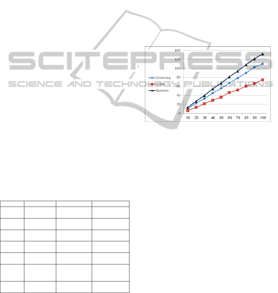
These results can be explained by the fact the Q-
learning algorithm's decision is based on the best
action achieved hitherto and a certain small proba-
bility of random choice while the Bayesian inference
algorithm considers several different normal distri-
butions of the student and therefore its performance
is much more accurate.
Figure 5: The average utility obtained by the different
algorithms as a function of the number of questions.
The results of the Gittins method were relatively
lower than the Bayesian algorithms, probably due to
the fact that the Gittins indices were calculated as-
suming independencies among the possible values,
and this assumption does not hold in our domain,
where the different levels are correlated. Neverthe-
less, the Gittins Indices' performance is relatively
high in comparison to most of the algorithms' per-
formances.
To summarize, when comparing the Gittins indi-
ces method and the Bayesian learning based algo-
rithm, we can note the following points:
1. Both methods assume normal distributed arms or
alternatives.
2. The Gittins indices takes into account future
rewards as a result of the exploration of new
arms, considering an infinite horizon scope, giv-
en a constant discount ratio, while the Bayesian
inference algorithm maximizes the expected util-
ity of the next step.
3. The Bayesian learning algorithm considers the
correlation between different alternatives, while
ICAART2014-InternationalConferenceonAgentsandArtificialIntelligence
252
the Gittins based algorithm assumes independent
arms.
In fact, when comparing both methods, the Bayesian
based algorithm outperforms the Gittins based algo-
rithm, However, the Gittins Indices' performance is
relatively higher than most of the algorithms' per-
formances, given more than 10 steps. Moreover, the
Gittins algorithm is the best one when considering
high levels of improvement of the student level, as
illustrated in Figure 8.
Note also that if the normal distribution does not
hold, the UCB algorithm (Auer, Cesa-Bianchi and
Fischer, 2002) can be applied for multi armed bandit
processes. In contrast to Gittins method, the UCB
algorithm considers a finite set of actions, but again,
the alternative arms are assumed to be independent,
while in our study, a correlation does exists, as ex-
plained in point 3 above.
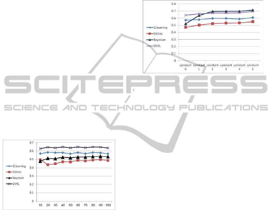
Next we compare the rate of successes in answer-
ing a question as shown in Figure 6. As observed,
the DVRL and the Q-learning methods achieve the
highest rate of success in answering question. But,
since they achieve a relatively low average of utility,
one can infer that these methods tend to offer easy
questions relative to the optimal level of questions
that should be provided.
Figure 6: The rate of questions that were successfully
answered as a function of the number of questions in the
simulation.
Note that the rate of success of the Bayesian can
also be increased by assigning higher weights for
correctly answering a question. For example, this
can be done by assigning a negative utility for a
question answered incorrectly, as provided in Utility
function #2, which is defined in Section 3:
question i=1..N
(level
i
+ C | question i was correctly answered) –
question i=1..N
(C | question
i was not correctly answered).
According to this utility function, for each cor-
rectly answered question the student receives a posi-
tive constant C (reward) in addition to the question's
level. However, for any incorrectly answered ques-
tion the student receives a constant negative value C
(penalty).
Consequently, next we compare all proposed algo-
rithms when the following utility function is used to
calculate the performance of the various algorithms
as presented in Figure 7.
Figure 7: The rate of questions correctly answered w.r.t.
all questions that were asked, as a function of the constant
C taken in the utility function (ITS with 50 questions).
As can be seen in Figure 7, for the simulations
considering the above utility function with a con-
stant higher than 2 (i.e., the value of 2 for the reward
and -2 for the penalty), and with 50 questions a tu-
toring session, the Bayesian algorithm achieves the
highest accuracy level.
The explanation can be due to the fact that the
policy of the Q learning family algorithms, and in
particular the policy of DVRL, is careful, and for the
most part they prefer to choose the well-known suc-
cessful choice rather than explore new possibilities.
Thus, they chose relatively low level questions,
which achieve higher success rates but with lower
total utilities.
However, as the successfulness of question an-
swering has a higher effect on the utility function,
the Bayesian learning method, which aims to max-
imize the utility function, also suggests low level
questions to obtain higher utility values, and thus the
rate of successful questions increases respectively.
Thus we can conclude that the choice of the utili-
ty function has a great impact on the algorithms'
performances and further research should be con-
ducted in educational arena to verify which utility
function ideally represents the success of an ITS
when taking into account the teachers' and the stu-
dents' preferences that will allow the utmost effi-
ciency of the ITS.
Another interesting matter is the effect of stu-
dents who improve their abilities over time. In order
to test the performance of the different algorithms in
this case, we assumed that a mean threshold level for
AdaptationSchemesforQuestion'sLeveltobeProposedbyIntelligentTutoringSystems
253

each student will increase with constant rate after
each step of the simulation.
Figure 8 demonstrates that for runs of 50 ques-
tions, where the mean level of the student is im-
proved each step by =0.05, and for more improve-
ment, the Gittins algorithm outperforms all other
algorithms, including the Bayesian inference meth-
od.
Figure 8: The algorithms' average utility for given im-
provements in the student's level during time.
However, an improvement level of d=0.05 means
that after 50 questions, a relative weak student (with
an average level of 2) will become an almost excel-
lent student (with an average level of 4.5), and in
real environments, such an improvement does not
occur so quickly.
The reason behind this lies in the fact that the
Gittins based algorithm may return to non beneficial
arms when their usage becomes relatively low (since
the Gittins indices depends on the usage of the arm),
and thus, the Gittins based algorithm does not ignore
the improvement of the student, and gives ITS the
ability to present harder questions as the student's
level improves. Future research is needed to include
the student's level of improvement in the model
considered by the Bayesian learning algorithm.
8 CONCLUSIONS
In this paper we examine different RL algorithms
that decide how to learn students' ability and how to
adapt the level of the question to the student's abil-
ity. We examined different algorithms, including Q
learning, TD, VRL, DVRL, Gittins' indices and
Bayesian inference, and we found that the Bayesian
inference based algorithm achieved the best results.
Moreover, the Q-learning based algorithm, named
DVRL, achieved the highest success rate.
The advantage of the Bayesian inference based
algorithm lie in the fact that it considers all the alter-
native distributions for each student, and updates its
beliefs regarding all the alternatives after each step.
The conclusion from this paper is that it may be
worthwhile to integrate the Bayesian inference based
algorithm as a Reinforcement Learning method in
future Intelligent Tutoring Systems.
However, these results are limited to artificial en-
vironments with simulated students. In future work
we intend to compare the Bayesian inference algo-
rithm using real data on the distribution of student
levels. Moreover, we intend to implement the Bayes-
ian inference based algorithm in a real ITS by prac-
ticing reading comprehension, to check its results on
real students, and compare the results obtained when
questions are chosen by the Bayesian inference algo-
rithms w.r.t. results obtained from a software provid-
ing random generated questions.
An additional area of research is to define a more
accurate utility function which will correctly reflect
the students' preferences from the automated soft-
ware.
Another direction of future work would be to take
into account the dynamic level of a student which
changes during the running of the ITS, and suggest
the appropriate model for the Bayesian algorithm to
handle this situation. This direction is important
when considering ITS which works with the same
students over a long period, since during the said
time period the student's level can change. Conse-
quently the appropriate adaptive algorithm should be
considered for such cases.
REFERENCES
Auer, P., Cesa-Bianchi, N. & Fischer, P., 2002, Finite-
time Analysis of the Multiarmed Bandit Problem, Ma-
chine Learning, 47, 235–256.
Azoulay-Schwartz, R., Katz, R. & Kraus, S. 2013, Effi-
cient Bidding Strategies for Cliff-Edge Problems, Au-
tonoumous agenst and multi-agent systems.
Azoulay-Schwartz, R., Kraus, S. & Wilkenfeld, J., 2004,
Explotation vs. Exploration in Ecommerce: Choosing
a Supplier in an Environment of Incomplete Infor-
mation, International Journal on Decision Support
Systems and Electronic Commerce 381, p. 1-18.
Beck, J. E., Woolf, B. P. & Beal, C. R. 2000, ADVISOR:
A machine learning architecture for intelligent tutor
construction. National Conference on Artificial Intel-
ligence.
Conitzer, V. & Garera, N., 2006, Learning algorithms for
online principal–agent problems and selling 1416
goods online, Proceedings of the International Con-
ference on Machine Learning, p. 209–216.
Gittins, J. C., 1989, Multi-armed Bandit Allocation Indi-
ces. John Wiley & Sons.
ICAART2014-InternationalConferenceonAgentsandArtificialIntelligence
254

Harmon, M. E. & Harmon, S. S., 1997, Reinforcement
Learning: A Tutorial. Publisher: Citeseer 1997. Vol-
ume: 21, Issue: 2.
Iglesias, A., Martínez, P., Aler, R. & Fernández, F. 2008,
Learning teaching strategies in an Adaptive and Intel-
ligent Educational System through Reinforcement
Learning. Applied Intelligence. Volume 31, Number 1.
p. 89-106.
Malpani, A., Ravindran, B., & Murthy, H., 2009, Person-
alized Intelligent Tutoring System Using Reinforce-
ment Learning. Twenty-Fourth International Florida
Artificial Intelligence Research Society Conferences.
Martin, K. N. & Arroyo, I., 2004, AgentX: Using Rein-
forcement Learning to Improve the Effectiveness of
Intelligent Tutoring Systems. Lecture Notes in Com-
puter Science, 2004, Volume 3220/2004, p. 564-572.
Rusell, S. & Norving, P., 1995, Artificial Intelligence, A
modern approach. Perntice hall, Inc.
Sarma, H., 2007, Intelligent Tutoring Systems Using Rein-
forcement Learning, A Thesis, Thesis Sreenivasa, In-
dian Institute of Technology, Madras.
Sarma, H., & Ravindran, B., 2007, Intelligent Tutoring
Systems using Reinforcement Learning to teach Autis-
tic students. Conference on Home/Community Orient-
ed ICT for the Next Billion (HOIT).
Sutton, R. S. & Barto, A. G., 2005, Reinforcement Learn-
ing: An Introduction. The MIT Press Cambridge, Mas-
sachusetts.
Vreind, N., 1997. Will reasoning improve learning? Eco-
nomics Letters, 55(1), p. 9–18.
Woolf, B. P., 2009, Building Intelligent Interactive Tutors
Student-centered strategies for revolutionizing e-
learning. Elsevier Inc.
AdaptationSchemesforQuestion'sLeveltobeProposedbyIntelligentTutoringSystems
255
