
1-D Temporal Segments Analysis for Traffic Video Surveillance
M. Brulin,
C. Maillet and H. Nicolas
Labri, University of Bordeaux, Talence, France
Keywords: Video Surveillance, Traffic, Temporal Segment, Behavior.
Abstract: Traffic video surveillance is an important topic for security purposes and to improve the traffic flow
management. Video surveillance can be used for different purposes such as counting of vehicles or to detect
their speed and behaviors. In this context, it is often important to be able to analyze the video in real-time.
The huge amount of data generated by the increasing number of cameras is an obstacle to reach this goal. A
solution consists in selecting in the video only the regions of interest, essentially the vehicles on the road
areas. In this paper, we propose to extract significant segments of the regions of interest and to analyze them
temporally to count vehicles and to define their behaviors. Experiments on real data show that precise
vehicle’s counting and high recall and precision are obtain for vehicle’s behavior and traffic analysis.
1 INTRODUCTION
For several years, traffic video-surveillance is under
fast development and is important for security
purposes and to improve the traffic flow
management (Kastrina et al., 2003); (Buch et al.,
2011); (Tian et al., 2011). The aim consists in the
extraction from the video data of information related
to the vehicles behaviors and to the traffic flow. In
order to be really efficient, such a video surveillance
system has to be fully automatic and able to provide
in real time information concerning the object’s
behaviors in the scene. Events of interest are
essentially: vehicles entering or exiting the scene,
vehicle collisions, accident, too fast (or too low)
vehicles' speed, stopped vehicles or objects
obstructing part of the road, vehicle’s classification
(car, trucks, bicycle, pedestrian …), objects in
forbidden areas, normal and abnormal trajectories or
for statistical purposes (estimation of the number of
vehicles, their average speed, and the number of
vehicles which change their traffic lane…) (Zhu et
al., 2000); (Yoneyama et al., 2005); (Rodriguez and
Garcia, 2010). This requires obtaining information
concerning the vehicle’s texture and contours
(Bissacco et al., 2004), motion (Adam et al., 2008),
trajectories and speed (Stauffer, 2003).
To reach the real-time constraint while keeping
efficient analysis, the computational cost has to be
reduced. For that purpose, two solutions can be
investigated. A first solution is to reduce as much as
possible the computational load of the motion
estimation and object based segmentation
algorithms, with the risk to get sub optimal
estimations. A second solution consists in the
reduction of the amount of video data which has to
be treated. This solution appears to be interesting for
traffic video surveillance applications for which
large parts of the images do not contain any
interesting information.
In this context, a first solution is to define the
region of interest (ROI) in the images. For traffic
video surveillance, these areas correspond generally
to the road areas. The other parts of the images are
useless and can be eliminated. Frame skipping is
also a potential solution. Nevertheless, the increased
temporal distance does not simplify the spatio-
temporal analysis. If these solutions are interesting,
they are not sufficient to reduce sufficiently the
amount of original data which have to be analyzed.
In order to better reach our goal, it is necessary to
take into account the kind of information really
useful for the vehicle’s behavior analysis, i.e., the
trajectories and the size of the moving vehicles. A
promising solution consists in the extraction of the
temporal evolution of selected spatial segments (or
scanlines) in the image (Malinovski et al., 2009);
(Zhu et al., VISITRAM). Such 1-D segments
represent a very low amount of data and can
therefore be quickly analyzed. If they are chosen
wisely they can contain enough information
concerning the moving vehicles to allow an analysis
557
Brulin M., Maillet C. and Nicolas H..
1-D Temporal Segments Analysis for Traffic Video Surveillance.
DOI: 10.5220/0004733905570563
In Proceedings of the 9th International Conference on Computer Vision Theory and Applications (VISAPP-2014), pages 557-563
ISBN: 978-989-758-003-1
Copyright
c
2014 SCITEPRESS (Science and Technology Publications, Lda.)

of their behavior. In this paper, we propose a method
to choose efficiently these segments and to analyze
them in order to obtain relevant objects based
descriptors useful for vehicle’s behaviors analysis
and counting of vehicles.
2 TEMPORAL SEGMENT
PROPERTIES FOR TRAFFIC
VIDEOSURVEILLANCE
For video traffic surveillance applications, the
regions of interest (ROI) are mainly the road areas.
In most cases, these ROI are structured by
circulation lanes, on which vehicles are circulating.
The temporal evolution of segments included in
these ROI contains relevant information for traffic
analysis purposes. For each segment, an image,
called here Temporal Segment Image (TSI), is built
by accumulating a given segment along time. Fig. 1
shows two examples of TSI obtained with segments
parallel and perpendicular to the circulation lanes. In
the following, and for a better visualization of the
TSI, the perspective effect is compensated using a
rectangle (in the 3-D space) defined by parallel
circulation lanes. Figs. 2 and 5 show examples of
such a compensation. Their main characteristics are
the following:
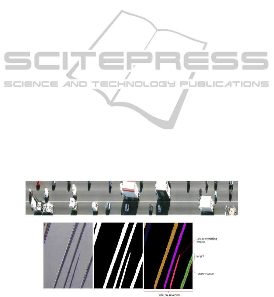
- Segments parallel to the circulation lanes: It can
be observed that each moving vehicle is represented
in the TSI by a band starting generally from the
bottom left to the top right of the image (see Fig. 1
bottom). The number of bands characterizes the
number of vehicles which overlap the segment in the
2-D space. The speed and acceleration of each
vehicle is obtained by computing the first and
second order derivatives of the contours of each
band. If the speed is constant, the band is a straight
line and its orientation gives the vehicle speed. At a
given time t, the length of the band represents the
vehicle’s length or height depending on the camera
orientation. The band may not be defined from the
bottom to the top of the image if the vehicle changes
its traffic lane. The dominant color of the band is
generally the dominant color of the vehicle.
- Segment perpendicular to the circulation lanes:
The number of vehicles can be counted by
segmented the image. The segmentation process is
easier than in the original image due to the fact that
the road areas in the TSI represent at each time
instant the same physical segment. Its texture is
more stable thereby facilitating the segmentation
process.
TSI based on segments parallel to the circulation
lanes contain more immediately available
information than TSI based on perpendicular
segments and contain most of information needed to
count and characterize vehicle’s behaviors. They are
therefore been used here. Nevertheless, some aspects
are missing such as information needed to identify
individually each vehicle such as the plates or the
vehicle’s models.
3 PROPOSED METHOD
The general block diagram of the proposed method
is shown in Fig. 3. It is decomposed into two main
stages: The first one is a pre-processing phase which
consists in the estimation of the scene background,
the detection of the circulation lanes, and the
selection of the road segments used to construct the
TSI. The second one consists in the TSI analysis in
real-time for vehicle’s behavior identification and
counting. Two assumptions are done: The camera is
assumed to be fixed and more or less oriented along
the main road axis. They are most of the time
reasonably fulfilled for traffic videosurveillance
cameras.
3.1 Pre-Processing Phase
The scene background is obtained using a per pixel
Gaussian mixture model (Bouwmans et al., 2008).
Modeling the history of pixel values by several
distributions helps the method to be more robust
against illumination changes or foreground moving
objects. The parameters of the mixture (weight w,
mean μ and covariance σ) are updated dynamically
over time. The probability P of occurrence of a color
u at the current pixel p and time t is given as (with k
the Gaussian number):
,
,,
,
,
,,
,
,,
,
,
,,
,
,,
is the i th Gaussian model. For
computational reason, RGB color components are
assumed to be independent, therefore the covariance
matrix
,,
is assumed to be diagonal, with
,,
as
its diagonal elements. At the beginning of the
system, only one Gaussian is initialized with a
predefined mean
(pixel value in the first image),
a high variance
and a low prior weight
. For
each new image and for each pixel, the first step
consists in determining the closest corresponding
VISAPP2014-InternationalConferenceonComputerVisionTheoryandApplications
558

Gaussian of the model using a k-mean approach.
Each pixel is matched to a given Gaussian k using
the Mahalanobis distance defined by
,
,
,
μ
,,
,,
,
μ
,,
The closest Gaussian is selected if 2.5.The
parameters of the selected Gaussian k are updated
as:
,,
1
,,
μ
,,
1
μ
,,
,
,,
1
,,
,
μ
,,
,
μ
,,
Fixed coefficients and are used to manage the
mean and covariance matrix update. For the non-
selected Gaussians only the weight is updated:
,,
1
,,
1
With c empirically fixed to 0.1. If a Gaussian is not
selected during a given period of time, its weight
becomes negative and it is suppressed. It is therefore
useless to fix a maximum Gaussian number. is
updated faster for new created Gaussians with are
less stable than Gaussians build with many
observations. Then we take: 1/.
With n the number of pixels used to build the
Gaussian. Finally, for each pixel, the background is
computed using the Gaussian with the highest w/
ratio. A pixel for which a different Gaussian has
been selected is considered as a foreground pixel. A
morphological filtering is done to fill small holes
and eliminated isolated ones. Using the background,
the road areas are estimated using a color criterion.
The circulation lanes are then detected on the road
areas using a method based on the CHEVP
algorithm. First, a Canny edge detector is applied.
Then, straight lines parameters are estimated using
the Standard Hough Transform. The vanishing point
is estimated by using the intersections of the
estimated lines as follows:
arg
∈
∑
,
∈
Where I is the set of intersections. J is the smallest
circle in the image plane which includes all
intersection points. Estimated lines which do not
cross the circle C centered on VP are eliminated.
The beam circle is empirically fixed at 10% of the
image width. This creates a segmentation of the ROI
into circulation lanes (see Fig. 4). Experiments show
that most of the circulation lines are correctly
estimated. For each couple of neighborhood lines, a
segment is automatically chosen on the line located
at equal distance between them, and on the lower
part of the road area in the image (see Fig. 4).
3.2 TSI Classification, Analysis
and Application
The goal of the segmentation is to separate the
foreground from the background areas in each TSI
by classifying each pixel as Foreground or
background. At each time instant, a new segment
is added to each TSI. Each pixel in
has therefore
to be classified knowing the segmentation obtained
for the previous segments. This is done using the
following algorithm:
- Temporal prediction: By construction, the pixels
located on the same horizontal line of a TSI
represent the same physical point along time
(considering that the camera is fixed). Segment
at time t-1 is then projected at time t using the
following rules: Each sub-segment labeled as
Foreground at time t-1 is projected at time t
assuming that there is no acceleration and using the
estimated speed for this object (see below). The rest
of the segment is predicted as background areas.
- Spatial Segmentation: the Gaussian mixture
method presented in Section 3.1 is also used to
obtain a pixel-based classification of
with the two
labels Foreground (F) or Background (B). A 1-D
morphological operator is applied to eliminate
isolated Foreground or Background pixels. Using
this pixel-based classification, each sub-segment
defined by a sliding window w is labeled as
Foreground if
∈/
∈/
S(p) denotes the label of pixel p. The length of w is
defined by the average length of a vehicle. This
length is computed as the average length of each
band in the past frames. This allows defining
foreground subsegments. Pixels at their boundaries
initially classified as Background pixels are
recursively eliminated from the Foreground sub-
segments to obtain the final spatial foreground
segments.
- Final labeling: The final labeling is obtained using
the following rules:
1- Overlapped sub-segments labeled as Foreground
in the two cases: They obviously correspond to
Foreground areas. The corresponding spatial
segment is therefore labeled as Foreground. This
allows tracking a vehicle by automatically detect
vehicle’s band in the TSI (see Figs. 1 and 2).
1-DTemporalSegmentsAnalysisforTrafficVideoSurveillance
559

2- Subsegments classified as Foreground by the
temporal prediction which do not overlap any spatial
foreground subsegment is not considered as a
foreground area at time t. It means that a vehicle has
disappear from the circulation lane.
3- Subsegments classified as Foreground by the
spatial analysis which do not overlap any temporal
foreground sub segment is considered as a new
vehicle (creation of a new vehicle’s band in the
TSI).
4- The rest of segment
is classified as
Background.
2.2 TSI Analysis and Application
The TSI images are analysis for traffic analysis as
follows:
- Vehicle’s speed estimation: For each detected
vehicle’s band, a line defined, for each time t, by the
middle of the band is built. The vehicle’s speed at
time t is obtained by the spatial derivate of this line.
If the vehicle is moving with a constant speed, a
straight line is obtained.
- Detection of traffic congestion: A traffic
congestion is detected if the average speed becomes
lower than a given threshold (values fixed by the
users) of the normal speed.
-Detection of stopped vehicles: If a line becomes
horizontal, it means that the vehicle has stopped (a
threshold defined by the users can be fixed to
consider the line as horizontal).
- Vehicle’s counting: The number of vehicles is
defined by the number of vehicle’s band. This is
done only if no traffic congestion is detected.
- Detection of overtaking vehicles: Case 2 and 3 in
the above classification method correspond
theoretically to a vehicle appearing or disappearing
from a lane. It corresponds directly to the number of
incomplete bands in the TSI.
4 EXPERIMENTAL RESULTS
The proposed method has been tested on a corpus
containing 25 videos (with temporal length from 10
to 30 minutes) of real videosurveillance data
obtained on various highways with variable weather
and lighting conditions (it includes videos acquired
during the night). After the pre-processing phase, all
experiments are obtained in real-time. It should also
be pointed out that the quality of the perspective
correction method is not critical for the TSI analysis
phase. The results are the following:
- Detection of traffic congestion: It is well detected
in all cases available in our corpus. Fig. 5 shows an
example. When the vehicles are moving very slowly
or are stopped, their relative distance is reduced and
their bands may merge. For this reason, it is difficult
to count vehicles in this situation. In that case, the
vehicle’s counting process is cancelled.
-Detection of stopped vehicles: Stopped vehicles
have been systematically detected in the few cases
available in our corpus (see Figs. 5 and 6).
- Vehicle’s counting: a recall of 94% and a precision
of 87 % are obtained (average results for each
circulation lane). The main problems arise with
trucks covering two (or more) circulation lanes in
the 2-D space mainly when the orientation of the
camera is not sufficiently along the circulation lanes.
As a consequence, they may be counted twice.
- Detection of overtaking vehicles: a recall of 97%
and a precision of 89 % are obtained.
Based on these analysis phases, more complete
vehicle’s behaviors can be detected. This is done
using a chronological analysis of the detected
events. Fig. 6 gives a typical example acquired in a
tunnel. In the considered video, a vehicle stops in the
middle of road. A truck which follows it has to
overtake the stopped vehicle, and came back in its
line when it is done. Finally the stopped vehicle
starts to move again. All of these events have been
correctly and automatically detected in the correct
chronological order as follows:
- Entrance in the scene of a first truck (Fig. 5a)
- Entrance of a second vehicle (a car, Fig. 5b)
- Detected stop of this car on the circulation lane
(Fig. 5c)
- Apparition of a third vehicle
- Disappearance of this vehicle before arriving near
the stopped vehicle (Fig. 5d)
- Apparition of the same vehicle in the TSI of the
second circulation lane (not shown in the figure)
- Disappearance of this vehicle from the second
circulation lane
- Apparition of this vehicle behind the stopped
vehicle (Fig. 5e)
- The stopped vehicle restarts (Fig 5f).
5 CONCLUSIONS
AND PERSPECTIVES
The approach described in this paper proposes a new
method to count vehicles and analyzed their
behaviors in real-time for traffic analysis purposes.
It is based on the analysis of the temporal evolution
VISAPP2014-InternationalConferenceonComputerVisionTheoryandApplications
560
of segments included and parallel to the circulation
lanes. It allows counting vehicles, to detect traffic
congestions, stopped vehicles and the detection of
vehicles overtaken. An application can be used to
characterize some more complex vehicles behaviors.
The approach has been validated on real video data
and in real-time in the context of traffic video
surveillance.
Several perspectives of this work are under
development such as: the detection of smaller
vehicles such as motorcycles or bicycles, a better
management of vehicles projected on two lanes due
to the perspective effect, and the definition of typical
complex scenarios useful for traffic
videosurveillance to automatically detect it on the
basis of a chronological analysis of the basic
descriptors estimated here.
REFERENCES
V. Kastrina, M. Zervakis and K. Kalaitzakis. A survey of
video processing techniques for traffic applications.
Image and Vision Computing, Vol. 21, N°4, pp. 359-
381, 2003.
N. Buch, S. A. Velastin and J. Orwell. A review of
computer vision techniques for the analysis of urban
traffic. IEEE Transactions on Intelligent
Transportation system, Vol. 12, N°3, pp. 920-939,
2011.
B. Tian, Q. Yao, Y. Gu, K. Wang and Y. Li. Video
processing techniques for traffic flow monitoring: A
survey. In Proc. of Int. Conf. on Intelligent
Transportation Systems, pp. 1103-1108, 2011.
Z. Zhu, G. Xu, B. Yang, D. Shi and X. Lin. VISATRAM: A
real-time vision system for automatic traffic
monitoring. Image and Vision Computing, Vol. 18,
No. 10, pp.781-794, 2000.
A. Yoneyama, C. H. Yeh and C. C. J. Kuo. Robust vehicle
and traffic information extraction for highway
surveillance. Image and Vision Computing, Vol.
2005, pp. 2305-2321, 2005.
T. Rodriguez and N. Garcia. An adaptive, real-time, traffic
monitoring system. Machine Vision and Applications.
Vol. 21, No. 4, pp. 555-576, 2010.
A. Bissacco, P. Saisan and S. Soatto. Gait recognition
using dynamic affine invariant. In int. Symposium on
Mathematical Theory of Network, and Systems. 2004.
A. Adam, E. rivlin, I. Shimshoni and D. Reinitz. Robust
real-time unusual event detection using multiple fixed-
location monitors. IEEE Trans. on Pattern Analysis
and Machine Intelligence, Vol. 30, N°3, pp.555-560,
2008.
C. Stauffer. Estimating tracking sources and sinks. In
Proc. of Computer Vision and Pattern Recognition,
IEEE, Vol. 4, pp.35-45, 2003.
Y. Malinovski, Y. Wang and Y.J. Wu. Video-based
vehicle detection and tracking using spatio-temporal
maps. Proc. of the Annual Transportation Research
Board meeting, Washington DC, 2009.
Z. Zhu, G. Xu, B. Yang, D. Shi and X. Lin. VISITRAM:
A real time vision system for automatic traffic
monitoring.
Bouwmans, T., El Baf, F. and Vachon, B., Background
modeling using mixture of gaussians for foreground
detection - A survey. Recent Patents on Computer
Science, pp. 219-237, 2008.
APPENDIX
Figure 1: Top: 1-D segment perpendicular to the circulation lanes. Bottom: 1-D segment parallel to the circulation lane.
Horizontal axis: temporal axis. Vertical axis: Segment axis.
1-DTemporalSegmentsAnalysisforTrafficVideoSurveillance
561
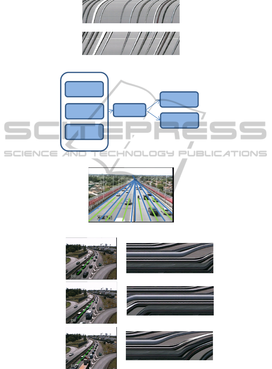
Figure 2: TSI before (top) and after (bottom) the perspective effect compensation.
Figure 3: Block diagram of the proposed method.
Figure 4: Estimated lanes and vanishing point (blue), chosen segments (green).
Figure 5: Examples in which traffic congestion has been automatically detected.
Sans correction perspective
Avec correction perspective
Circulationlane
detection
Choiceofthe
segments
Countingof
Vehicles
Background
estimation
TSI
construction
Vehicle’s
behavior
VISAPP2014-InternationalConferenceonComputerVisionTheoryandApplications
562
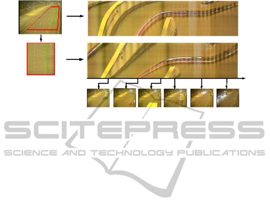
(a) (b) (c) (d) (e) (f)
Figure 6: Top: original image and the TSI corresponding to the green line. The red square is used for the perspective
compensation. Middle TSI after perspective correction. Bottom: original images illustrating the successive events.
1-DTemporalSegmentsAnalysisforTrafficVideoSurveillance
563
