
A New Two-Degree-of-Freedom Space Heating Model for Demand
Response
Anita Sant’Anna
1
and Robert Bass
2
1
Embedded and Intelligent Systems Research Group, Halmstad University, Halmstad, Sweden
2
Department of Electrical & Computer Engineering, Portland State University, Portland, OR, U.S.A.
Keywords:
Space Heating, Demand Response, Thermal Comfort, Thermodynamic Model, Simulation.
Abstract:
In today’s fast changing electric utilities sector demand response (DR) programs are a relatively inexpensive
means of reducing peak demand and providing ancillary services. Advancements in embedded systems and
communication technologies are paving the way for more complex DR programs based on transactive control.
Such complex systems highlight the importance of modeling and simulation tools for studying and evaluating
the effects of different control strategies for DR. Considerable efforts have been directed at modeling thermo-
statically controlled appliances. These models however operate with only one degree of freedom, typically,
the thermal mass temperature. This paper proposes a two-degree-of-freedom residential space heating system
composed of a thermal storage unit and forced convection system. Simulation results demonstrate that such
system is better suited for maintaining thermal comfort and allows greater flexibility for DR programs. The
performance of several control strategies are evaluated, as well as the effects of model and weather parameters
on thermal comfort and power consumption.
1 INTRODUCTION
The electric utilities sector currently faces a number
of challenges: how to manage electricity prices in an
unregulated market (Spees and Lave, 2007), how to
cope with more distributed and intermittent genera-
tion such as wind power (Kondoh et al., 2011), as
well as how to cope with ever increasing peak de-
mands (Ericson, 2009). Demand response (DR) pro-
grams are an effective means for alleviating such is-
sues. When consumers can respond in real time to
high electricity prices, they naturally tend to reduce
peak-time usage, and consequently help equalize de-
mand and prices (Spees and Lave, 2007). In addi-
tion, DR programs provide a more flexible and effi-
cient option for fast-response ancillary services (Kon-
doh et al., 2011).
Albadi et al. concisely summarized a hierarchy
of current incentive- and price-based utility DR pro-
grams (Albadi and El-Saadany, 2007). Incentive-
based residential programs often take the form of di-
rect control, wherein a utility can directly apply an
on/off duty cycle to customer appliances in order to
adjust aggregate customer demand. Often, such pro-
grams are used for load shedding during high-demand
periods. In return for taking part in such programs
customers are rewarded with an incentive, such as a
discount on their electricity bill. Incentive-based DR
has been considered in works such as (Mohsenian-
Rad et al., 2010).
Price-based programs, on the other hand, persuade
customers to change their electricity consumption be-
havior by adjusting prices throughout day. Price ad-
justments occur either in response to current demand
or are based on a predetermined time-of-use sched-
ule. Participating customers may therefore avoid
high electricity prices by modifying their behavior,
such as reducing consumption during peak-periods.
Price-based DR has been considered in works such as
(Fuller et al., 2011).
Current developments in embedded system tech-
nologies and communications make it possible to im-
plement home energy management (HEM) systems
that not only react to but also interact with the grid
through mechanisms like transactive control (Schnei-
der et al., 2011), (Chassin et al., 2008). In the future,
distributed HEM systems will be an integral part of
DR programs (Pipattanasomporn et al., 2012). Mod-
eling and simulation tools are essential in understand-
ing and evaluating the effects of different DR control
strategies prior to large scale deployment. In this con-
text, it is important to create residential load models
5
Sant’Anna A. and Bass R..
A New Two-Degree-of-Freedom Space Heating Model for Demand Response.
DOI: 10.5220/0004734600050013
In Proceedings of the 3rd International Conference on Smart Grids and Green IT Systems (SMARTGREENS-2014), pages 5-13
ISBN: 978-989-758-025-3
Copyright
c
2014 SCITEPRESS (Science and Technology Publications, Lda.)

that simulate the physical behavior of appliances par-
ticipating in DR programs (Shao et al., 2013).
Thermostatically controlled appliances (TCA),
such as water heaters and HVAC systems, are of par-
ticular interests because they can store thermal en-
ergy. Intelligent control strategies can make use of
this storage capacity in order to avoid operating dur-
ing peak periods with little inconvenience to the cus-
tomer. A 2001 survey by the Office of Energy Mar-
kets and End Use (RECS, 2001) reported that 9.1% of
household electricity consumption was due to water
heaters. Another considerable amount, 10.1%, was
due to space heating. Several pilot programs have
been conducted that employ hot water heaters as the
DR appliance, particularly in the U.S. states of Wash-
ington and Oregon (Kondoh et al., 2011), (Chassin
et al., 2008), (Diao et al., 2012), as well as in Norway
(Saele and Grande, 2011).
Considerable efforts have been directed to model-
ing thermostatically controlled loads. The thermody-
namic behaviors of electric water heaters and HVAC
system are normally described by differential equa-
tions (Lu, 2012), (Du and Lu, 2011), (Molina-Garcia
et al., 2011). Often, the system presents two behav-
iors: on or off. When the appliance is on, the temper-
ature of the thermal mass increases following a nega-
tive exponential curve (c − e
−τ
); when then appliance
is off, the temperature of the thermal mass decreases
exponentially (c + e
−τ
) (Lu et al., 2005). The time
constant τ relates to the thermal capacitance of the
thermal mass.
However, the above mentioned models present
only one degree of freedom (DoF) for control, typi-
cally, the desired indoor temperature or the minimum
and maximum acceptable temperatures for the ther-
mal mass (Pipattanasomporn et al., 2012). This pa-
per introduces a two-DoF space heating model com-
posed of a heat pump, a thermal storage unit (hot wa-
ter tank) and a forced convection system. The heat
pump transfers thermal energy to the thermal storage
and heats up the water. The hot water is circulated
through coiled pipes, transferring heat to it surround-
ing air, which is in turn circulated through the house
by the forced convection system. Such systems con-
tain, in effect, two thermal masses: the thermal stor-
age unit and the thermal mass of the house (air and
structures). These systems are not new, they are com-
mon in Canada and in Nordic countries, however, they
have not yet been considered in DR studies.
This paper demonstrates that two-DoF systems
are better adapted for maintaining thermal comfort
and allow greater flexibility for DR programs. The
DR performance of the proposed system is compared
to a traditional one-DoF system through simulations.
The systems are evaluated with respect to their ability
to maintain indoor temperature within a comfortable
range (Peeters et al., 2009). Simple control strategies
are proposed for the forced convection system cou-
pled to on-off, and multistage compressors. Simula-
tion results show the importance of considering two-
DoF models for DR.
The contributions of this paper may be summa-
rized as follows.
• The description of a two-DoF heating system
model composed of an insulated thermal storage
unit and a forced convection system (FCS);
• The comparison and evaluation of two-DoF and
one-DoF systems for price-based DR;
• The evaluation of different control strategies for
two-DoF systems, and their effect on thermal
comfort for on/off, and multistage compressors as
well as three different weather profiles;
The remainder of the paper is organized as fol-
lows. Thermodynamic model and control strategies
are described in Section 2. Model and simulation pa-
rameters used for the study are explained in Section 3.
Simulation results are presented in Section 4 and dis-
cussed in Section 5. Finally, Section 6 concludes this
paper.
2 MODELS
2.1 Thermodynamic Model
The proposed system consists of:
• A rectangular volume with insulated walls repre-
senting the house.
• An insulated thermal energy storage unit (hot wa-
ter tank).
• A heat pump directly coupled to the thermal mass.
• A forced convection system (FCS) that transfers
heat from the thermal mass to the house.
This thermodynamic model can be represented as
a thermal circuit, as shown in Figure 1. The equiv-
alent mathematical model is shown in Equation (2),
where T
H
is the indoor temperature; T
TM
is the ther-
mal mass temperature; and T
O
is the ambient outdoor
temperature. The mass of the water in the storage
tank is m
TM
and its specific heat is C
TM
. The heat
storage capacity of the house is represented by the
capacitance of value C
H
m
H
, which includes the heat
capacity of the air contained in the house as well as
it’s structure and materials. The heat conductivity be-
tween the thermal mass and the house is represented
SMARTGREENS2014-3rdInternationalConferenceonSmartGridsandGreenITSystems
6

Figure 1: Thermal circuit representation of the thermody-
namic model. T
H
is the indoor temperature; T
TM
is the ther-
mal mass temperature; and T
O
is the ambient outdoor tem-
perature. The mass of the water in the storage tank is m
TM
and its specific heat is C
TM
. The heat storage capacity of
the house is represented by the capacitance of value C
H
m
H
,
which includes the heat capacity of the air contained in the
house as well as it’s structure and materials. The heat con-
ductivity between the thermal mass and the house is repre-
sented by Y
T M−H
, which depends on the heat transfer coef-
ficient created by the FCS, Y
FC
, and the thermal mass heat
loss, Y
L
, according to equation 1. The conductivity of the
house insulation is represented by K
H
; and
˙
Q
HP
is the heat
pump’s thermal power output.
by Y
T M−H
, which depends on the heat transfer coeffi-
cient created by the FCS, Y
FC
, and the thermal mass
heat loss, Y
L
, according to Equation 1. The conductiv-
ity of the house insulation is represented by K
H
; and
˙
Q
HP
is the heat pump’s thermal power output.
It is worth noting that, if the conductivity between
the thermal mass and the house Y
T M−H
is kept con-
stant, this model is qualitatively no different from pre-
viously proposed models (Lu, 2012), (Du and Lu,
2011), (Molina-Garcia et al., 2011). However, by
considering an insulated thermal mass coupled with
a FCS, the indoor temperature is introduced as a new
degree of freedom, in addition to the temperature of
the thermal mass.
Y
T M−H
= Y
FC
+Y
L
(1)
˙
T
H
=
K
H
(T
O
− T
H
) −Y
TM-H
(T
H
− T
TM
)
m
H
C
H
(2a)
˙
T
TM
=
˙
Q
HP
−Y
TM-H
(T
TM
− T
H
)
m
TM
C
TM
(2b)
2.2 Forced Convection System Model
and Control
Consider a FCS that can operate in two fan speed
modes, low and high. The two modes are modeled as
different heat transfer coefficients between the ther-
mal mass and the house, Y
FC-low
and Y
FC-high
respec-
tively. The output of the FCS is controlled by a set of
if-then rules based on the ambient indoor temperature,
T
H
, as shown in Equation (3). The total heat transfer
between the thermal mass and the house is computed
from Equation 1.
Y
FC
=
0 if T
H
>T
H-goal
Y
FC-low
if T
H-goal
−1<T
H
≤T
H-goal
Y
FC-high
if T
H
≤T
H-goal
−1
(3)
2.3 Heat Pump Model and Control
We consider a multistage heat pump capable of three
modes of operation: low, medium and high. The ther-
mal power supplied by each operation mode will be
referred to as
˙
Q
HP-low
,
˙
Q
HP-med
and
˙
Q
HP-high
respec-
tively.
In order to avoid modeling a short-cycled com-
pressor, we assume that the heat pump may not be
switched on and off in less than 5 minutes.
Operation is also affected by the demand response
program, which requires the pump to switch off dur-
ing peak periods, represented by the time-of-use rate
TUR
on-peak
.
Four different control scenarios are considered:
• Case I: A traditional one-DoF system where the
indoor temperature is directly coupled to the ther-
mal storage temperature, and consequently, to the
heat pump output. The heat transfer coefficient
between the thermal mass and house is constant,
Y
TM-H
= Y
FC-low
+ Y
L
. This scenario considers a
heat pump with only on/off operation. The heat
pump output is controlled based on the indoor
temperature as shown in Equation (4).
˙
Q
HP
=
{
0 if T
H
>T
H-goal
or TUR
on-peak
˙
Q
HP-high
if T
H
≤T
H-goal
−1
(4)
• Case II: A simple two-DoF system where the in-
door temperature and the thermal storage temper-
ature are controlled separately. The FCS is re-
sponsible for regulating the indoor temperature
and the heat pump is responsible for regulating the
thermal mass temperature. The heat pump is ei-
ther on or off, and its output is controlled based on
the thermal mass temperature as shown in Equa-
tion (5). The FCS operates as shown in Equa-
tion (3).
ANewTwo-Degree-of-FreedomSpaceHeatingModelforDemandResponse
7

˙
Q
HP
=
{
0 if T
TM
>T
TM-goal
or TUR
on-peak
˙
Q
HP-high
if T
TM
≤T
TM-goal
−2
(5)
• Case III: This scenario considers the previous
two-DoF system but with a multistage heat pump
that can operate in three different modes: low,
medium or high. The operation mode selection is
done through a collection of if-then rules based on
the thermal mass temperature as shown in Equa-
tion (6). The FCS operates as shown in Equa-
tion (3).
˙
Q
HP
=
0 if T
TM
>T
TM-goal
or TUR
on-peak
˙
Q
HP-low
if T
TM-goal
−1<T
TM
≤T
TM-goal
˙
Q
HP-med
if T
TM-goal
−3<T
TM
≤T
TM-goal
−1
˙
Q
HP-high
if
T
TM
≤T
TM-goal
−3
(6)
• Case IV: This final scenario considers the pre-
vious two-DoF system with a multi-stage heat
pump. The heat pump output selection, however,
is done with the help of a PD controller as shown
in Equation (7). The FCS operates as shown in
Equation (3).
˙
Q
ctrl
= k
P
(T
TM-goal
− T
TM
) + k
D
˙
T
TM
(7a)
˙
Q
HP
=
0 if
˙
Q
ctrl
≤
˙
Q
HP-low
or TUR
on-peak
˙
Q
HP-low
if
˙
Q
HP-low
<
˙
Q
ctrl
≤
˙
Q
HP-med
˙
Q
HP-med
if
˙
Q
HP-med
<
˙
Q
ctrl
≤
˙
Q
HP-high
˙
Q
HP-high
if
˙
Q
ctrl
>
˙
Q
HP-high
(7b)
2.4 Thermal Comfort
Acceptable upper and lower temperatures for residen-
tial buildings, as suggested by Peeters et al. (Peeters
et al., 2009), are given by Equations (8a) and (8b),
respectively, where T
n
is the indoor temperature, w is
the width of the comfort band in
◦
C, and α is a con-
stant ≤ 1. The study suggests that w = 5 and α = 0.7
incur in 90% acceptability. T
n
is computed as shown
in Equation (8c), where T
O−avrg
is the daily average
of the ambient outdoor temperature. The total time (in
hours) during which the indoor temperature is ourside
the comfort band, t
Disc
, can be computed as shown in
Equation (9), where i indicates each simulation time
step and J is the duration of the simulation time step in
seconds. Variations in temperature also affect thermal
comfort. Regarding cycling temperature, ASHRAE
standard 55-2004 (ANSI/ASHRAE 55-2004, 2004)
states that, if the peak variation exceeds 1.1
◦
C, the
rate of temperature change shall not exceed 2.2
◦
C/h.
T
upper
= T
n
+ wα (8a)
T
lower
= T
n
− w(1 − α) (8b)
T
n
= 20.4 + 0.06 T
O-avrg
(8c)
Disc(i) =
{
0 if T
lower
≤T
H
(i)≤T
upper
1 if T
H
(i)<T
lower
or T
H
(i)>T
upper
(9a)
t
Disc
=
J
3600
24(3600/J)
∑
i=1
Disc(i) (time in hours) (9b)
2.5 Power Usage and Cost Assessment
The electric power, P
HP
, consumed by the heat pump
at every simulation time step, i, is computed us-
ing Equation (10), relating heat transfer to electrical
power consumption via the heat pump coefficient of
performance (COP). The total cost, C
total
, for oper-
ating the system for one day can be computed based
on the time of use rates (TUR), as shown in Equa-
tion (11). Where J is the duration of the simulation
time step in seconds. Electricity consumption by the
FCS is not included in the cost analysis.
P
HP
(i) =
˙
Q
HP
(i)
COP(
˙
Q
HP
(i),T
O
(i))
(10)
C
total
=
24(3600/J)
∑
i=1
P
HP
(i)TUR(i)T (11)
3 SIMULATION SETTINGS
3.1 Model Parameters
We consider a 600 m
3
house (21188.8 cubic feet). The
heat capacity of the house, C
H
m
H
= 37968 kJ.K
−1
,
includes the heat capacity of its structure and vol-
ume of air. The heat capacity of the air con-
tained in the house was calculated from its vol-
ume, density (1.2041 kg.m
−3
), and specific heat
(1.005 kJ.kg
−1
.K
−1
). The heat capacity of the house
SMARTGREENS2014-3rdInternationalConferenceonSmartGridsandGreenITSystems
8
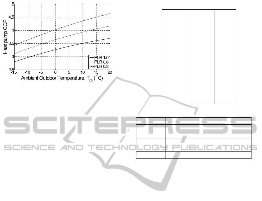
Figure 2: Heat pump coefficient of performance (COP) as a
function of ambient outdoor temperature, T
O
, and part-load
ratio (PLR).
structure was calculated based on the method de-
scribed in (Olsen and Rode, 2008); considering Gyp-
sum plasterboard walls and ceilings 0.05 m thick, and
concrete and tile flooring 0.1 m thick.
We consider a thermal storage unit of 150 gal-
lons (approximately 568 L). The thermal capacitance
of the thermal storage unit, C
TM
m
TM
= 2376 kJ.K
−1
,
was calculated from its volume, the density of wa-
ter (1.00 kg.L
−1
), and the specific heat of water
(4.185 kJ.kg
−1
.K
−1
). The thermal conductance of
the storage insulation, Y
L
= 0.003 kW.K
−1
, was calcu-
lated based on the typical electric water heater proper-
ties described in (DOE, 1998) (Table 8); considering
a cylindrical storage of 35 inches in diameter.
The heat transfer coefficient related to the insu-
lating properties of the house, K
H
= 0.2530 kW.K
−1
,
derives from the surface area and thermal resistivity
of the home, and was calculated using the Oak Ridge
National Laboratory Online Simple Whole Wall R-
value Calculator (www.ornl.gov).
The heat transfer coefficients used for the FCS,
Y
TM-H
, was derive from Equation (2a), considering
there is no heat exchange with the outside, i.e. K
H
=
0; and the thermal mass is at a constant 65
◦
C. The
values for Y
FC-high
and Y
FC-low
were chosen so as to
increase the indoor temperature from 16 to 20
◦
C in
30 and 60 minutes respectively.
We consider a three-ton multistage heat pump,
adopting a COP model from Jeter et al. (Jeter et al.,
1987) that allows for COP to vary as a function
of both ambient outside temperature and compressor
speed. COP ranges represent a typical multi-speed
heat pump. The three operation modes,
˙
Q
HP-low
,
˙
Q
HP-med
and
˙
Q
HP-high
, correspond to 0.3, 0.6 and 1
part-load ratios (PLR) respectively. Figure 2 shows
the COP curves for each PLR.
The target indoor temperature, T
H-goal
, was 21
◦
C.
This temperature is the approximate center of comfort
Table 1: Model parameters.
parameter value unit
C
TM
m
TM
2 376 kJ/K
C
H
m
H
37 968 kJ/K
K
H
0.2530 kW/K
Y
FC-high
1.800 kW/K
Y
FC-low
0.900 kW/K
Y
L
0.003 kW/K
˙
Q
HP-low
3.15 kW
˙
Q
HP-med
6.30 kW
˙
Q
HP-high
10.5 kW
T
H-goal
21
◦
C
T
TM-goal
65
◦
C
k
P
1 kW/K
k
D
5 kJ/K
Table 2: Time of use rates for winter months.
time rate [cents/kWh]
on-peak
06:00 to 10:00
13.266
17:00 to 20:00
mid-peak
10:00 to 17:00
7.500
20:00 to 22:00
off-peak 22:00 to 06:00 4.422
range for the chosen weather profiles. The target ther-
mal mass temperature, T
TM-goal
, was 65
◦
C, which is
high enough to kill harmful bacteria in the water, but
not so high as to risk scalding in case of accident.
Model parameter values are summarized in Ta-
ble 1.
3.2 Simulation Parameters
The TUR reflect the winter rates in use by Portland
General Electric, as shown in Table 2, and were ap-
plied equally to all three locations. Three weather
profiles are considered: the average hourly tempera-
tures for January 1st in Portland, OR; Halmstad, Swe-
den; and Colorado Springs, CO; as shown in Figure 3.
Temperature control cases I through IV are simu-
lated for each of the three outdoor temperature pro-
files. The demand response program requires the
heat pump to switch off during peak time-of-use rates
(TUR). Total power usage and cost were calculated
for each scenario. Initial values for T
H
and T
TM
were
21 and 65
◦
C respectively. The chosen simulation
time step J is 60 seconds, and the total simulation time
is 24 hours. Simulations are performed using Acumen
(www.acumen-language.org) (Taha et al., 2011), a
modeling language where models are defined through
differential equations and simulations are generated
automatically.
ANewTwo-Degree-of-FreedomSpaceHeatingModelforDemandResponse
9
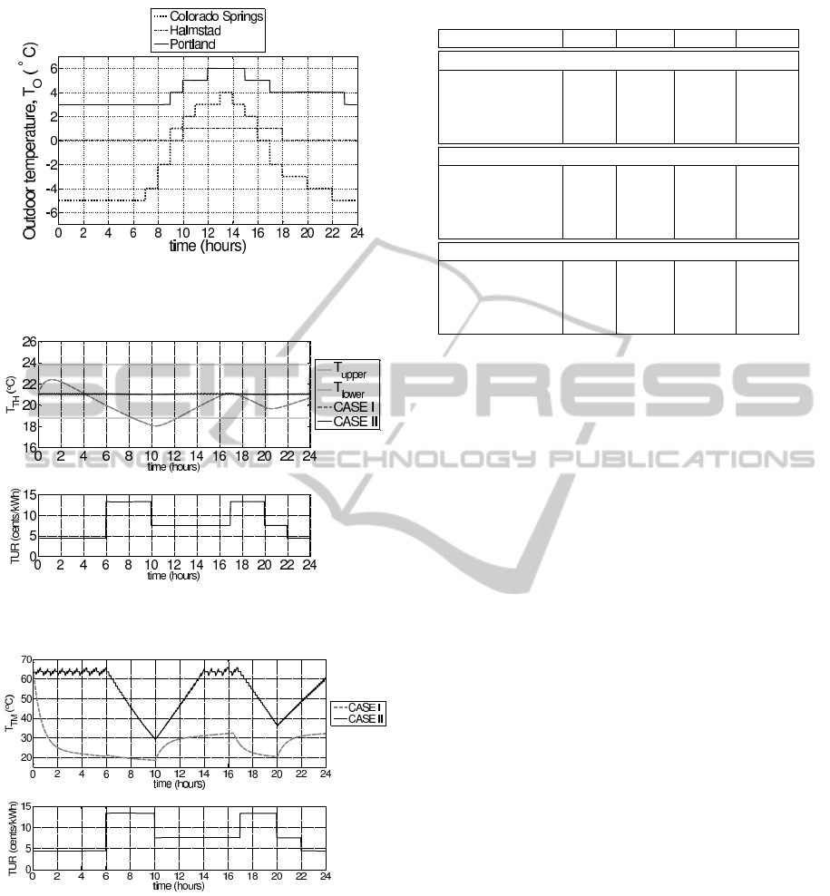
Figure 3: Weather profiles for Portland, Colorado Springs
and Halmstad. Average hourly outdoor temperature for the
month of January in each of the locations.
Figure 4: Indoor temperature, T
H
, and time-of-use rates
(TUR) for cases I and II, Colorado Springs weather profile.
Figure 5: Thermal mass temperature, T
TM
, and time-of-use
rates (TUR) for cases I and II, Colorado Springs weather
profile.
4 RESULTS
Control cases I and II represent a typical one-DoF
system and the proposed two-DoF system respec-
tively, both under similar on/off control strategies.
The simulation results for indoor and thermal mass
temperature, contrasting these two cases under the
Table 3: Thermal comfort.
Case I Case II Case III Case IV
Colorado Springs
t
Disc
[hours] 4.02 0 0 0
mean T
H
[
◦
C] 20.11 21.02 21.02 21.01
cyclic ∆T
H
[
◦
C] 4.37 0.12 0.12 0.10
cyclic
˙
T
H
[
◦
C/h] 0.58 - - -
Halmstad
t
Disc
[hours] 1.45 0 0 0
mean T
H
[
◦
C] 20.44 21.03 21.02 21.02
cyclic ∆T
H
[
◦
C] 3.79 0.12 0.12 0.10
cyclic
˙
T
H
[
◦
C/h] 0.50 - - -
Portland
t
Disc
[hours] 0 0 0 0
mean T
H
[
◦
C] 20.66 21.04 21.03 21.03
cyclic ∆T
H
[
◦
C] 3.29 0.12 0.12 0.10
cyclic
˙
T
H
[
◦
C/h] 0.60 - - -
Colorado Springs weather profile, are shown in Fig-
ures 4 and 5 respectively. Very similar results were
obtained for simulations under Halmstad and Portland
weather profiles.
Results show that the response of the one-DoF
system (Case I) varies greatly and slowly. The in-
door temperature starts considerably high because the
initial thermal mass temperature is 65
◦
C. The ther-
mal mass temperature must decrease considerably in
order to maintain the indoor temperature within the
comfortable range. Another drawback of the one-DoF
system is that during peak-hours, when the heat pump
is off, the temperature of the house falls considerably
below the limits of thermal comfort Figure 4. The
additional DoF introduced by the FCS (Case II) al-
lows the thermal mass temperature to vary consider-
ably from 65 down to approximately 30
◦
C, Figure 5,
while the indoor temperature strays very little from
the goal temperature of 21
◦
C, Figure 4.
A summary of the indoor temperature results for
each of the simulated scenarios is shown in Table 3.
Note that the traditional one-DoF system simulated in
Case I results in indoor temperatures outside the com-
fortable limits for both Colorado Springs and Halm-
stad weather profiles. The two-DoF system simulated
in Cases II through IV, on the other hand, maintain the
indoor temperature very close to 21
◦
C with less than
0.2
◦
C of peak-to-peak cyclic variations.
Figure 6 shows the heat pump output, Q
HP
, and
thermal mass temperature, T
TM
, for cases II through
IV for the Colorado Springs weather profile. In all
cases, the thermal mass temperature profile is very
similar. Case II shows slightly larger cyclic oscilla-
tions due to the on/off duty cycles. The same pat-
terns were observed for simulations under Halmstad
and Portland weather profiles.
A summary of the thermal mass temperature be-
SMARTGREENS2014-3rdInternationalConferenceonSmartGridsandGreenITSystems
10
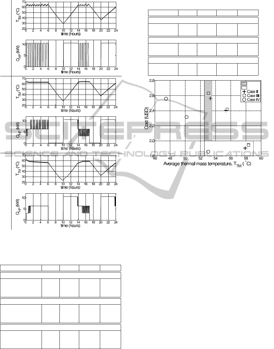
CASE IICASE IIICASE IV
Figure 6: Thermal mass temperature, T
TM
, and heat pump
output, Q
HP
, for cases II though IV, Colorado Springs
weather profile.
Table 4: Thermal storage.
Case I Case II Case III Case IV
Colorado Springs
max T
TM
[
◦
C] 65.00 65.69 65.00 65.00
min T
TM
[
◦
C] 18.37 28.99 27.76 22.95
mean T
TM
[
◦
C] 26.15 53.32 53.07 47.48
Halmstad
max T
TM
[
◦
C] 65.00 65.78 65.00 65.00
min T
TM
[
◦
C] 19.13 31.08 32.14 26.90
mean T
TM
[
◦
C] 26.02 55.36 55.53 50.19
Portland
max T
TM
[
◦
C] 65.00 65.78 65.14 65.00
min T
TM
[
◦
C] 19.65 36.93 37.70 31.98
mean T
TM
[
◦
C] 25.34 57.91 58.35 53.04
havior for all control cases is shown in Table 4. Note
that the mean temperatures for Case I are consider-
ably below the intended temperature of 65
◦
C.
Table 5: Power consumption and cost.
Case I Case II Case III Case IV
Colorado Springs
Power [kWh] 33.447 41.940 42.806 40.935
Cost [USD] 2.31 2.56 2.63 2.56
Halmstad
Power [kWh] 30.312 37.726 42.806 35.858
Cost [USD] 2.07 2.40 2.63 2.31
Portland
Power [kWh] 23.543 29.505 30.364 28.502
Cost [USD] 1.57 1.90 1.94 1.85
Figure 7: Average thermal mass temperature versus cost
for control cases II, III, and IV. The gray box highlights
that cases I and II incur a cost of approximately 2,6 USD
to maintain a mean temperature of about 53
◦
C, whereas
case IV maintains the same mean temperature for only 1,85
USD. The clear box highlights that control cases II and III
are able to achieve an average temperature approximately
5
◦
C higher than case IV for an increased cost of less than
0,10 USD.
The power usages and costs for each simulated
scenarios are shown in Table 5. Case I consumes con-
siderably less energy than the other cases, however,
it does not fulfill the thermal comfort requirements.
Figure 7 shows a plot of mean thermal mass temper-
ature against cost for control cases II through IV un-
der all three weather profiles. The gray box in Fig-
ure 7 highlights that cases I and II incur a cost of ap-
proximately 2,6 USD to maintain a mean temperature
of about 53
◦
C, whereas case IV maintains the same
mean temperature for only 1,85 USD. Note also that
control cases II and III are able to achieve an aver-
age temperature approximately 5
◦
C higher than case
IV for an increased cost of less than 0,10 USD, high-
lighted by the clear box in Figure 7.
ANewTwo-Degree-of-FreedomSpaceHeatingModelforDemandResponse
11

5 DISCUSSION
The proposed two-degree-of-freedom system pro-
vides more flexibility for DR programs. By decou-
pling the heat pump output from the indoor temper-
ature, the thermal storage can be used to store more
energy, as evidenced by the higher thermal mass tem-
peratures for Cases II through IV. The direct coupling
of the heat pump output and the indoor temperature in
Case I suggests that there is need for more advanced
predictive control strategies, specifically ones that can
pre-heat the structure in anticipation of peak time-of-
use rates or extreme weather. Such predictive control,
however, would not be able to cope with accidental
power loss or other unforeseeable issues. Having a
thermal storage, able to operate at higher tempera-
tures, makes the system more robust and more flex-
ible.
Simulation results show that a heat pump operates
at maximum output when switching on immediately
after peak pricing hours end. This occurs because the
heat pump must compensate for the large thermal en-
ergy loss incurred during peak pricing hours. This
reconnection effect may increase power consumption
overall, and shift the peak periods instead of lessening
them. The effects of reconnecting appliances after a
forced disconnection has been studied, e.g. (Ericson,
2009), and control strategies have been designed to
minimize this reconnection effect for water heaters,
e.g. (Nehrir et al., 1999). In the case of space heating,
the reconnection spike may be reduced by making the
controller aware of current and predicted weather, or
pre-heating in anticipation of peak TUR. Reconnec-
tion costs and mitigating strategies will be investi-
gated in future works.
It is important to note that the control strategies
proposed here were not optimized in any way. Lower
goal temperatures for the thermal mass, for example,
are likely to result in lower power consumption. How-
ever, we implemented very simple and intuitive con-
trollers for the purpose of comparing different control
strategies that resulted in similar thermal mass and
house temperature profiles. There are many research
opportunities for optimization schemes that take into
account real-time pricing, weather predictions, and
other factors.
This paper investigates the behavior of single iso-
lated systems, where the only outside inputs were
weather and time-of-use rates. This facilitated an un-
derstanding of system properties. The next step is
to understand the impact of thousands of such sys-
tems being used for DR. Monte Carlo methods can be
used to simulate a large number of these systems with
slightly different parameters so as to model the slight
differences between real houses. However, in order to
develop a practical system model, parameters must be
validated against practical experiments. Future works
will focus on more realistic and large scale simula-
tions.
Customer willingness to participate in DR pro-
grams increases as the benefits they derive exceed the
cost of the inconvenience (Fahrio
˜
glu and Alvarado,
2000). Minimizing or eliminating discomforts should
lead to increased participation in such programs. De-
spite the simplifications made in this study, our re-
sults show that an insulted thermal storage unit cou-
pled to a heat pump and forced convection system
for space heating may be used in price-based demand
response programs without either compromising the
thermal comfort of the residents nor requiring they
modify their behavior by deferring consumption to a
later time period. This proposed system, therefore,
could be a means by which to increase participation
levels within utility DR programs.
6 CONCLUSION
Demand response programs are effective and rela-
tively inexpensive ways to cope with peak demands;
balance demand and generation; and stabilize elec-
tricity prices. Water heaters and HVAC systems
are commonly used for DR. This paper introduces a
space heating system composed of an insulated ther-
mal mass and forced convection system with two de-
grees of control freedom that can be used for DR. The
thermodynamic model was presented as well as four
different temperature control strategies. Simulations
were used to evaluate the performance of the sys-
tem based on thermal comfort and power consump-
tion in three different weather regions. Results show
that the FCS introduces an important degree of free-
dom that improves indoor temperature control while
at the same time allowing the temperature of the ther-
mal mass to vary more freely. The power consump-
tion of the system can vary greatly according to the
control strategy and the insulating properties of the
house. Future research avenues include investigat-
ing optimized control strategies that account for real-
time pricing, weather forecasts, occupancy patterns,
among others; and, investigating the aggregate de-
mand response of large numbers of homes equipped
with heat pumps, forced convection and controllable
thermal masses.
SMARTGREENS2014-3rdInternationalConferenceonSmartGridsandGreenITSystems
12

ACKNOWLEDGEMENTS
Partial funding for this research was provided by Port-
land General Electric (PGE). PGE played no role in
the design and analysis of the study, nor the interpre-
tation of findings. Nor did PGE participate in the writ-
ing of this report or the decision to submit this article
for publication.
REFERENCES
Albadi, M. and El-Saadany, E. (2007). Demand response
in electricity markets: An overview. In Power Engi-
neering Society General Meeting, 2007. IEEE, pages
1 –5.
ANSI/ASHRAE 55-2004 (2004). Thermal environmental
conditions for human occupancy. ASHRAE 55-2004.
ANSI Approved.
Chassin, D., Hammerstrom, D., and DeSteese, J. (2008).
The pacific northwest demand response market
demonstration. In Power and Energy Society General
Meeting - Conversion and Delivery of Electrical En-
ergy in the 21st Century, pages 1–6.
Diao, R., Lu, S., Elizondo, M., Mayhorn, E., Zhang, Y.,
and Samaan, N. (2012). Electric water heater mod-
eling and control strategies for demand response. In
Power and Energy Society General Meeting, 2012
IEEE, pages 1 –8.
DOE (1998). Results and methodology of the engineering
analysis for residential water heater efficiency stan-
dards. US Department of Energy, Office of Codes and
Standards.
Du, P. and Lu, N. (2011). Appliance commitment for house-
hold load scheduling. Smart Grid, IEEE Transactions
on, 2(2):411–419.
Ericson, T. (2009). Direct load control of residential water
heaters. Energy Policy, 37(9):3502 – 3512.
Fahrio
˜
glu, M. and Alvarado, F. (2000). Designing incen-
tive compatible contracts for effective demand man-
agement. Power Systems, IEEE Transactions on,
15(4):1255 –1260.
Fuller, J., Schneider, K., and Chassin, D. (2011). Analy-
sis of residential demand response and double-auction
markets. In Power and Energy Society General Meet-
ing, 2011 IEEE, pages 1–7.
Jeter, S., Wepfer, W., Fadel, G., Cowden, N., and Dymek, A.
(1987). Variable speed drive heat pump performance.
Energy, 12(12):1289 – 1298.
Kondoh, J., Lu, N., and Hammerstrom, D. (2011). An eval-
uation of the water heater load potential for providing
regulation service. Power Systems, IEEE Transactions
on, 26(3):1309 –1316.
Lu, N. (2012). An evaluation of the hvac load potential for
providing load balancing service. Smart Grid, IEEE
Transactions on, 3(3):1263–1270.
Lu, N., Chassin, D., and Widergren, S. (2005). Model-
ing uncertainties in aggregated thermostatically con-
trolled loads using a state queueing model. Power Sys-
tems, IEEE Transactions on, 20(2):725–733.
Mohsenian-Rad, A.-H., Wong, V., Jatskevich, J., Schober,
R., and Leon-Garcia, A. (2010). Autonomous
demand-side management based on game-theoretic
energy consumption scheduling for the future smart
grid. Smart Grid, IEEE Transactions on, 1(3):320–
331.
Molina-Garcia, A., Kessler, M., Fuentes, J., and Gomez-
Lazaro, E. (2011). Probabilistic characterization of
thermostatically controlled loads to model the impact
of demand response programs. Power Systems, IEEE
Transactions on, 26(1):241–251.
Nehrir, M., LaMeres, B., and Gerez, V. (1999). A customer-
interactive electric water heater demand-side manage-
ment strategy using fuzzy logic. In Power Engineering
Society 1999 Winter Meeting, IEEE, volume 1, pages
433 –436 vol.1.
Olsen, L. and Rode, C. (2008). Heat capacity in relation
to the danish building regulation. In Proceedings of
the 8th Symposium on Building Physics in the Nordic
Countries: Selected papers, volume 3, pages 16–18.
Peeters, L., de Dear, R., Hensen, J., and D’haeseleer, W.
(2009). Thermal comfort in residential buildings:
Comfort values and scales for building energy simu-
lation. Applied Energy, 86(5):772 – 780.
Pipattanasomporn, M., Kuzlu, M., and Rahman, S. (2012).
An algorithm for intelligent home energy manage-
ment and demand response analysis. Smart Grid,
IEEE Transactions on, 3(4):2166–2173.
RECS (2001). Residential energy consumption surveys. US
Energy Information Administration, Office of Energy
Markets and End Use.
Saele, H. and Grande, O. (2011). Demand response
from household customers: Experiences from a pilot
study in norway. Smart Grid, IEEE Transactions on,
2(1):102 –109.
Schneider, K., Fuller, J., and Chassin, D. (2011). Anal-
ysis of distribution level residential demand response.
In Power Systems Conference and Exposition (PSCE),
2011 IEEE/PES, pages 1–6.
Shao, S., Pipattanasomporn, M., and Rahman, S. (2013).
Development of physical-based demand response-
enabled residential load models. Power Systems, IEEE
Transactions on, 28(2):607–614.
Spees, K. and Lave, L. B. (2007). Demand response and
electricity market efficiency. The Electricity Journal,
20(3):69 – 85.
Taha, W., Brauner, P., Cartwright, R., Gaspes, V., Ames,
A., and Chapoutot, A. (2011). A core language for
executable models of cyber physical systems: work in
progress report. SIGBED Rev., 8(2):39–43.
ANewTwo-Degree-of-FreedomSpaceHeatingModelforDemandResponse
13
