
Precise Phase Measurements using an Entangled Coherent State
P. A. Knott
1
and J. A. Dunningham
1,2
1
School of Physics and Astronomy, University of Leeds, Leeds LS2 9JT, U.K.
2
Department of Physics and Astronomy, University of Sussex, Falmer, Brighton BN1 9QH, U.K.
Keywords:
Coherent State, Metrology, Phase Measurement.
Abstract:
Quantum entanglement offers the possibility of making measurements beyond the classical limit, however
some issues still need to be overcome before it can be applied in realistic lossy systems. Recent work has
used quantum Fisher information (QFI) to show that entangled coherent states (ECSs) may be useful for this
purpose as they combine sub-classical phase precision capabilities with robustness (Joo et al., 2011). However,
to date no effective scheme for measuring a phase in lossy systems using an ECS has been devised. Here we
present a scheme that does just this. We show how one could measure a phase to a precision significantly better
than that attainable by both unentangled ‘classical’ states and highly-entangled NOON states over a wide range
of different losses. This brings quantum metrology closer to being a realistic and practical technology.
1 INTRODUCTION
Quantum metrology is the art of making precision
measurements by taking advantage of the properties
of quantum mechanics. The main advantage of quan-
tum metrology over classical metrology is that it al-
lows us to achieve the same precision with fewer re-
sources. Making more precise measurements with
limited numbers of particles or photons has many
important applications, including microscopy, grav-
itational wave detection, measurements of material
properties, and medical and biological sensing (Na-
gata et al., 2007). Many of these examples could ben-
efit from a device which operates with a lower photon
flux, for example in biological sensing, where dis-
turbing the system too much can damage the sam-
ple. Another important reason for developing quan-
tum metrology is that it provides a stepping stone
to more complicated quantum technologies such as
quantum computers: if we can build metrological de-
vices that can beat the classical limit by exploiting
entanglement, then this puts us in a good position to
begin to tackle more advanced manipulations of quan-
tum properties. Furthermore, measurements are cru-
cial to the development of science, and any way to
improve them is a welcome development.
One of the main stumbling points in quantum
metrology is creating a state that is robust to particle
losses, which will always be a concern in any realistic
device. In this paper we present an optical state that
shows remarkable robustness to photon losses: en-
tangled coherent states ECSs. We discuss how these
states can be created, and present a scheme which
allows us to measure a phase using an ECS to sub-
classical precision, even when a wide range of differ-
ent loss rates are accounted for.
2 PRECISE PHASE
MEASUREMENTS
2.1 Enhancement using Entanglement
Throughout this paper we will generally be con-
cerned with measuring phases in a device using the
same principles of a Mach-Zehnder interferometer, as
shown in Fig. 1. The first step in this device is to
combine the two input states at a beam splitter. One
of the paths then picks up a phase, φ, and the two
paths are recombined at a second beam splitter. The
resulting output from the second beam splitter can be
measured by detectors D1 and D2 to extract the phase
information. A ‘classical-like’ state of light, which is
equivalent to sending a sequence of independent sin-
gle particles (SP) through the interferometer allows
one to measure the phase with a precision that scales
with the total number of particles n as the “shot noise
limit” 1/
√
n (Gkortsilas et al., 2012). However by
making use of an entangled state, the precision can be
205
Knott P. and Dunningham J..
Precise Phase Measurements using an Entangled Coherent State.
DOI: 10.5220/0004734902050211
In Proceedings of 2nd International Conference on Photonics, Optics and Laser Technology (PHOTOPTICS-2014), pages 205-211
ISBN: 978-989-758-008-6
Copyright
c
2014 SCITEPRESS (Science and Technology Publications, Lda.)
improved to 1/n: the “Heisenberg limit” (Dunning-
ham and Kim, 2006).
φ
D1
D2
Beam
Splitter
Beam
Splitter
Input 1
Input 2
Figure 1: A Mach-Zehnder interferometer which can be
used to measure a phase φ. Photons are send through the
beam splitters and phase shift, then measured at the detec-
tors D1 and D2.
In order to create an entangled number state we
replace the first beam splitter in the interferometer in
Fig. 1 by a “quantum beam splitter” (QBS). A quan-
tum beam splitter is like an ordinary interferometer,
but with a nonlinearity in one arm (Dunningham and
Kim, 2006) instead of the phase, and has the follow-
ing effect on state |n,0i:
|n,0i
QBS
−−→
1
√
2
[|n,0i+i|0,ni] (1)
The state on the right hand side is known as a
NOON state (Dowling, 2008). After creating the
NOON state, we then apply the phase shift to one
of the paths in the interferometer, as we did with the
SP state. We can then send this state through a sec-
ond QBS, and measure the number of particles at the
detectors. If we send a NOON state of n particles
through through this scheme, then the precision of
phase measurement can be seen to vary as δφ = 1/n,
the Heisenberg limit (Dunningham and Kim, 2006).
However, there is a problem with such an ap-
proach because NOON states are highly fragile to par-
ticle loss. Losing just one particle from a NOON
state (Eq. 1) will project the state onto either
e
inφ
|n,0i or i|0,ni. The global phase in each of
these cases is not physical and cannot be measured,
so all the phase information is lost when we lose
just one particle. Despite this, a number of clever
schemes have been devised with robustness to loss
which still capture sub shot noise limit precision, al-
beit not quite at the Heisenberg limit. An example of
one of these schemes is a NOON “chopping” strat-
egy (Dorner et al., 2009), in which multiple smaller
NOONs are sent through an interferometer instead
of one big one. Other examples include unbalanced
NOON states (Demkowicz-Dobrzanski et al., 2009),
BAT states (Gerrits et al., 2010) and mixtures of SP
and NOON states (Gkortsilas et al., 2012). While
these states can beat the shot noise limit when loss is
included, they are still fragile, and with large amounts
of loss they are outperformed by classical strategies.
We will now turn to a state which shows huge poten-
tial, as it is intrinsically robust to the effects of loss:
coherent states.
2.2 Entangled Coherent States
A coherent state is defined as:
|αi = e
−
|α|
2
2
∞
∑
n=0
α
n
√
n!
|ni, (2)
where α is a complex amplitude and n is the particle
number. In order to achieve quantum enhanced mea-
surement, we still need to create an entangled coher-
ent state (ECS) (Sanders, 2012; Hirota et al., 2011):
N
|α,0i+e
iθ
|0,αi
(3)
where N = 1/
p
2 +2e
−|α|
2
cosθ. We could create
the ECS with θ = π/2 by sending input state |α,0i
through the QBS. Alternatively, the ECS with θ = 0
can be created by interacting a “cat state” N
α
(|+αi+
|−αi) with a coherent state |αiat a beam splitter (Joo
et al., 2011). This latter scheme is likely to be more
experimentally feasible. However, the issue of exper-
imental implementations will be left to later work.
In order to investigate the potential of the ECS in
quantum metrology, Joo et. al. (Joo et al., 2011)
calculated its quantum Fisher information (QFI). The
QFI for a general state ρ (Braunstein and Caves, 1994;
Boixo et al., 2009) is given by:
F
Q
= Tr
ρA
2
(4)
where A is found from solving the symmetric loga-
rithmic derivative ∂ρ/∂φ = 1/2 [Aρ + ρA]. The preci-
sion in the phase measurement (more specifically the
lower bound on the standard deviation) is given by the
quantum Cram
´
er-Rao bound (Braunstein and Caves,
1994):
δφ ≥
1
p
µF
Q
, (5)
where µ is the number of copies of the state (i.e. times
that the measurement is independently repeated).
This gives the best possible precision with which a
state can measure a phase. For NOON states and SP
states the quantum Cram
´
er-Rao bound gives us the
Heisenberg and shot noise limits respectively.
Joo et. al. used the QFI to show that with and
without loss the ECS can achieve better precisions
than SP, NOON, and some other candidate states.
PHOTOPTICS2014-InternationalConferenceonPhotonics,OpticsandLaserTechnology
206
Zhang et. al. (Zhang et al., 2013) derived an ex-
pression for the QFI with loss for arbitrary α, and
confirmed the potential of ECSs for robust quan-
tum metrology. What is still missing, however, is a
concrete way for converting this promise into a real
scheme for making the phase measurement.
3 MEASURING A PHASE USING
AN ENTANGLED COHERENT
STATE
3.1 A Simple Scheme with No Loss
We will now look at the effect of sending input state
|ψ
1
i = |α,0i through the interferometer in Fig. 1, but
with the beam splitters replaced by QBSs. The effect
of the first QBS is to produce the ECS |ψ
2
i:
|ψ
1
i = |α,0i
QBS
−−→
1
√
2
(|α,0i+ i|0,αi) = |ψ
2
i. (6)
We then perform a phase shift which gives us the
state:
|ψ
3
i =
e
−
|α|
2
2
√
2
∞
∑
n=0
α
n
√
n!
e
inφ
|n,0i+i|0,ni
=
1
√
2
|αe
iφ
,0i+i|0,αi
, (7)
followed by the second QBS:
|ψ
4
i = e
−
|α|
2
2
∞
∑
n=0
α
n
√
n!
ie
inφ
2
|n,0isin
nφ
2
+ |0,nicos
nφ
2
.
From this we can calculate the probability ampli-
tude of detecting different numbers of photons at the
outputs. To do this we first take the inner product of
|ψ
4
i with |n
1
i
D1
|n
2
i
D2
= |n
1
,n
2
i, i.e. the state with n
1
photons at detector D1 and n
2
photons at detector D2.
This gives us:
hn
1
,n
2
|ψ
4
i =
ie
−
|α|
2
2
α
n
1
√
n
1
!
e
in
1
φ
2
sin
n
1
φ
2
δ
n
2
,0
+
α
n
2
√
n
2
!
e
in
2
φ
2
cos
n
2
φ
2
δ
n
1
,0
.
The delta functions here tell us that it is impossible
to detect photons at both outputs. This is clearly true
as any photon detection collapses the state into either
|n,0i or |0,ni. We can now calculate the probabilities
of different numbers of photons being detected, given
that the phase in the interferometer is φ
1
:
P(n
1
,n
2
|φ = φ
1
) =
|
hn
1
,n
2
|ψ
4
i
|
2
(8)
Using this conditional probability distribution we
can apply Bayesian statistics to build up our knowl-
edge of the phase φ as we repeat the process with a
stream of ECSs (Gkortsilas et al., 2012). Fig. 2 shows
that this scheme, with no loss, allows us to beat the
best possible precision obtainable using NOON states
of comparable sizes. For small α we do not saturate
the QFI, but we significantly improve upon the best
possible measurement using a NOON state. For large
α this scheme comes very close to saturating the QFI,
but it can be seen that in this region ECSs and NOON
states operate at a very similar precision.
1 2 3 4 5
0
0.005
0.01
0.015
0.02
0.025
0.03
0.035
0.04
α
δφ
δφ
CM
δφ
CF
δφ
NF
Figure 2: The phase precision of the scheme described in
section 3.1 for no loss is shown here. We plot different sized
ECSs against their precision. Here (and in later figures)
δφ
CM
is the ECS using our measurement scheme, δφ
CF
is
the QFI for the ECS and δφ
NF
is the QFI for the NOON
state (of equivalent size as each ECS). SP states measure at
precision 0.0354.
We will now briefly discuss the details of our
scheme that allow us to compare our results to NOON
and SP states. In many applications of quantum
metrology such as biological sensing, probing materi-
als properties and gravitational wave detection, we are
concerned with the number of photons (or particles)
passing through the phase shift itself, and would like
to minimise this number when possible. We would
therefore like to compare the phase measurement pre-
cision of different states when a set number of pho-
tons R enter the phase. For the unentangled state
we simply send the state through the interferometer
2R times, as in each run an average of 1/2 a pho-
ton enters the phase shift. For the NOON state in
equation 1, each run sends n/2 photons through the
phase shift, and so we simply send the NOON state
through the interferometer 2R/n times. For ECSs the
situation is slightly different, as each run contains a
different number of photons. We can calculate the av-
erage number of photons passing through the phase
for the general ECS in equation 3 to be ¯n = N
2
|α|
2
,
PrecisePhaseMeasurementsusinganEntangledCoherentState
207
and we therefore send the ECS through the interfer-
ometer R/¯n times. For most of our results we have
used R = 400 as this allows us to consistently cal-
culate the precision of the phase measurement with
different states.
3.2 Introducing Loss
Measurement by
the environment
BS
Fictional beam
splitter
Incoming
state
Figure 3: This shows a “fictional” beam splitter and mea-
surement by the environment as a model for loss.
To simulate the effects of loss we introduce “fictional”
beam splitters after the phase shift (Gkortsilas et al.,
2012; Joo et al., 2011; Demkowicz-Dobrzanski et al.,
2009) as shown in Fig. 3, which have probability of
transmission η ≡cos
2
θ. After the phase shift and in-
cluding the vacuum states used to simulate loss, the
ECS we are concerned with is given by:
|ψ
0
i =
1
√
2
|αe
iφ
,0,0,0i+i|0,0,α,0i
, (9)
where the second and fourth terms in the kets repre-
sent the modes into which particles are lost from the
first and third terms respectively.
The effect of the “fictional” beam splitters then
leaves us in the state |Ψ
1
i given by:
1
√
2
h
|αe
iφ
sinθ, αe
iφ
cosθ, 0,0i+i|0,0, αsin θ,α cos θi
i
.
We then take the density matrix ρ
1
= |ψ
1
ihψ
1
|
and to represent measurement by the environment we
trace over the environmental modes as follows:
ρ
2
=
∑
e
1
∑
e
2
he
1
|he
2
|ρ
1
|e
2
i|e
1
i. (10)
Using
∑
e
he|XihY |ei = hY |Xi and the
nonorthogonality of coherent states hα|βi =
exp(−
1
2
|α|
2
+ α
∗
β −
1
2
|β|
2
) it can be shown that
ρ
2
is reduced to:
ρ
2
= c
1
(|ψ
2
ihψ
2
|)+
1
2
c
2
|αe
iφ
√
η,0ihαe
iφ
√
η,0|+|0,α
√
ηih0,α
√
η|
where c
1
= e
|α|
2
(η−1)
, c
2
= 1 −c
1
and:
|ψ
2
i =
1
√
2
|αe
iφ
√
η,0i+i|0,α
√
ηi
. (11)
The resulting state is a mixture of loss and no loss
components. For NOON states we know during each
run if there has been loss simply by counting the num-
bers of particles at the outputs. However, for ECSs we
can no longer do this, as we don’t know the number
of particles in an ECS to begin with. This, combined
with the fact that the size of the coherent state has
decreased after the loss, means that the ECS in this
simple interferometer loses its phase precision more
quickly than NOON states, as shown in Fig. 4. This
agrees with the work by (Zhang et al., 2013) who cal-
culated the Fisher information of ECSs with loss for
any value of α. They showed that the quantum en-
hancement of the ECS decreases more quickly than
NOON states with loss. Despite this they also showed
that the ECSs still contain some phase information af-
ter loss (unlike NOON states) and this should allow
us to recover the phase information and therefore end
up beating NOON states in the long run. Our simple
scheme clearly does not do this, but in the next section
we will present a scheme that does.
0.5 0.55 0.6 0.65 0.7 0.75 0.8 0.85 0.9 0.95 1
0
0.01
0.02
0.03
0.04
0.05
0.06
0.07
η
δφ
δφ
NF
n=4
δφ
SF
δφ
CM
α=2
Figure 4: Here the legend refers to states as in Fig. 2, with
δφ
SF
the QFI for SP states. We can see that ECSs degrade
quickly with loss (α =
√
2 here). For larger α the ECS loses
precision with loss even quicker.
4 IMPROVED SCHEME WITH
LOSS
Despite the fact that an entangled coherent state can
still retain some phase information after loss, we
have seen that with a simple measurement scheme the
PHOTOPTICS2014-InternationalConferenceonPhotonics,OpticsandLaserTechnology
208
phase information cannot be recovered, and we end
up doing even worse than NOON states. We have de-
vised a scheme, shown in Fig. 5, which can be used to
recover this desired phase information. The key is to
use extra “reference” coherent states above and below
the main interferometer which can be used to perform
a homodyne measurement and recover the phase in-
formation. When a photon is lost from the ECS in
equation 7 the state collapses into |αe
iφ
,0i or |0,αi.
If we are left with the second state, then the phase in-
formation is irretrievable, but if we are left with the
state |αe
iφ
,0i then the phase information is still there.
However, in order to extract it we need a reference
state |αi to “compare” it to, hence including the up-
per and lower arms in our interferometer.
QBS
QBS
φ
D1
D3
BS
D2
BS
D4
Loss after the phase shift
Figure 5: Quantum interferometer with extra arms to re-
cover phase information with loss.
The state in this “long arm” interferometer after
the phase shift is:
|Ψ
1
i =
1
√
2
|α
1
,α
0
e
iφ
,0,α
1
i+i|α
1
,0,α
0
,α
1
i
(12)
= |Φ
1
i+|Φ
2
i. (13)
After being acted on by the fictional beam splitters
that simulate loss, this state is transformed from
|Ψ
1
i to |Ψ
2
i. We then trace over the environmental
degrees of freedom to give ρ
1
=
∑
e
he
2
|Ψ
2
ihΨ
2
|ei
where |ei represents all four environmental modes.
This gives us:
ρ
2
= |Φ
1η
ihΦ
1η
|+|Φ
2η
ihΦ
2η
| (14)
+ e
−|α
0µ
|
2
(|Φ
1η
ihΦ
2η
|+|Φ
2η
ihΦ
1η
|), (15)
where η is the transmission rate through the inter-
ferometer, |Φ
1η
i =
1
√
2
|α
1η
,α
0η
e
iφ
,0,α
1η
i, |Φ
2η
i =
i
√
2
|α
1η
,0,α
0η
,α
1η
i, α
0η
= α
0
√
η, α
1η
= α
1
√
η and
α
0µ
= α
0
√
1 −η. This state can also be written as:
ρ
2
= c
1
|Ψ
1η
ihΨ
1η
|+c
2
(|Φ
1η
ihΦ
1η
|+|Φ
2η
ihΦ
2η
|)
where |Ψ
1η
i is the state in equation 12 with all the
α reduced to
√
ηα. In this form it is easy to see that
the mixed state after loss is comprised of a pure state
|Ψ
1η
i with coefficient c
1
= e
−|α
0µ
|
2
, a collapsed state
|Φ
1η
i which contains the phase, and a collapsed state
|Φ
2η
i that does not contain the phase, both with coef-
ficient c
2
= 1 −c
1
. We can then send ρ
2
through the
remainder of the interferometer, giving the probabili-
ties at the outputs as:
P(#) = h#|Φ
1η
ihΦ
1η
|#i+h#|Φ
2η
ihΦ
2η
|#i
+ e
−|α
0µ
|
2
h#|Φ
1η
ihΦ
2η
|#i+h#|Φ
2η
ihΦ
1η
|#i
,
where |#i= |k, l,m,ni, the state with k particles in the
first output, l in the second and so on. The barred
states |Φ
1η
i and |Φ
2η
i can be found by sending |Φ
1η
i
and |Φ
2η
i through the remainder of the interferome-
ter. We initially took the obvious choice for the “refer-
ence” states as α
1
= α
0
. However, we found that this
scheme gave us poor results, as shown in Fig. 6 where
α =
√
2. For this very small choice of α
0
=
√
2 we
can beat the NOON and SP states up to around 15%
loss, which is indeed a very positive find. But after
this point it is more beneficial to use either NOON or
SP states. If we increase α then the results soon get
much worse and before long we cannot beat either
NOON or SP states if there is any loss at all.
0.4 0.5 0.6 0.7 0.8 0.9 1
0.01
0.02
0.03
0.04
0.05
0.06
0.07
η
δφ
δφ
CM
δφ
NF
δφ
SF
Figure 6: This scheme clearly doesn’t perform well com-
pared to NOON and SP when there is more than 15% loss.
Despite these shortcomings, the clear potential of
ECSs warranted a more rigorous search for changes
PrecisePhaseMeasurementsusinganEntangledCoherentState
209
that can optimise our scheme. Indeed, if we in-
stead use the initial ECS N (|α,0i + |0,αi) where
N = 1/
q
2(1 +e
−|α|
2
), as used by Joo et. al. (Joo
et al., 2011), we begin to get more positive results. A
much more significant change we can make is to vary
the size of α
1
for different loss values, in some cases
up to around α
1
= 2.4α
0
– a detailed study of why this
is the case is the subject of ongoing work. The pre-
cision with which this scheme can measure the phase
also depends on the (approximate) phase being mea-
sured (this is true for most schemes). Nonetheless this
should not pose much of a problem as we can just put
a variable phase shift in the lower-middle path, which
allows us to vary the phase difference so that effec-
tively φ can be whatever we choose.
0.3 0.4 0.5 0.6 0.7 0.8 0.9 1
0.02
0.03
0.04
0.05
0.06
0.07
η
δφ
δφ
CM
δφ
NF
δφ
SF
δφ
CF
Figure 7: With a large α
1
we can beat both the NOON and
SP states. Here, for α
0
=
√
2 we beat both NOON and SP
all of the time.
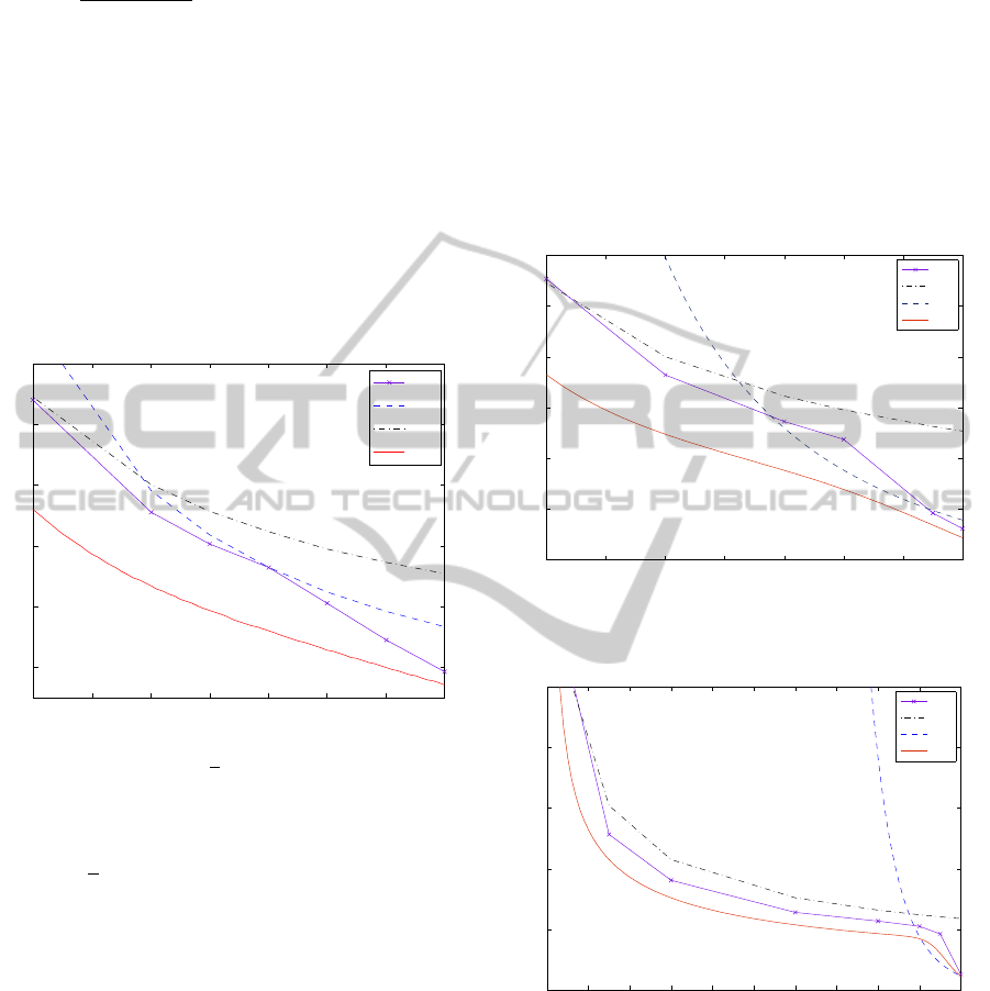
With these changes, and after carefully optimising
over φ and α
1
, we then obtain the results in Fig. 7
for α
0
=
√
2. It can be seen that our state now out-
performs the NOON and SP states for all values of
loss. Figures 8 and 9 show the results for α
0
= 2 and
α
0
= 5 respectively. We can see that for these larger
values of α
0
our scheme still beats the competitors for
the majority of η values.
Our results fit well with the Fisher information
given by Zhang et. al. which is shown as the red
solid line δφ
CF
on all three figures. The authors
showed that for large α there is a small region where
the NOON state performs better than the ECS be-
cause “although the classical term of the ECS is ro-
bust against the photon losses, the Heisenberg term
decays about twice as quick as that of the NOON
state” (Zhang et al., 2013). This agrees well with our
results. Our scheme doesn’t saturate the Fisher infor-
mation, but come reasonably close, and this is enough
to beat the NOON and SP states much of the time.
Future work will include examining different
ECSs with different QBSs in order to try and come
closer to saturating the QFI. We would also like to
look how this measurement scheme could be carried
out in an experiment. Despite the fact that we have
looked at how to measure the phase, there are still
parts of our scheme that are not easily achievable in
experiment, and we would like to iron these parts out
so that we have a fully realisable scheme to measure a
phase to a significantly higher precision that the com-
peting states.
0.3 0.4 0.5 0.6 0.7 0.8 0.9 1
0.01
0.02
0.03
0.04
0.05
0.06
0.07
η
δφ
δφ
CM
δφ
SF
δφ
NF
δφ
CF
Figure 8: Here α = 2. Our scheme beats NOON and SP
states for most loss values.
0 0.1 0.2 0.3 0.4 0.5 0.6 0.7 0.8 0.9 1
0
0.03
0.06
0.09
0.12
0.15
η
δφ
δφ
CM
δφ
SF
δφ
NF
δφ
CF
Figure 9: Here α = 5. Again we perform better than NOON
and SP most of the time.
5 CONCLUSIONS
Despite the Fisher information for entangled coherent
states showing great potential for robust phase mea-
surement, up to this point it has not been clear how
the phase information can actually be measured. Here
we show a scheme which can achieve this. When
PHOTOPTICS2014-InternationalConferenceonPhotonics,OpticsandLaserTechnology
210

there is no loss our scheme utilises entanglement to
perform sub-classical precision. More significantly,
we are also able to recapture phase information when
there has been loss. This is not possible with sin-
gle particle or NOON states, and so our results im-
prove upon these competitors for the majority of loss
rates. This work brings us ever closer to the ultimate
goal in quantum metrology of measuring a phase to a
sub-classical precision even when there are significant
losses in the system.
ACKNOWLEDGEMENTS
This work was partly supported by DSTL (contract
number DSTLX1000063869).
REFERENCES
Boixo, S., Datta, A., Davis, M., Shaji, A., Tacla, A.,
and Caves, C. (2009). Quantum-limited metrology
and Bose-Einstein condensates. Physical Review A,
80(3):032103.
Braunstein, S. and Caves, C. (1994). Statistical distance
and the geometry of quantum states. Physical Review
Letters, 72(22):3439–3443.
Demkowicz-Dobrzanski, R., Dorner, U., Smith, B., Lun-
deen, J., Wasilewski, W., Banaszek, K., and Walms-
ley, I. (2009). Quantum phase estimation with lossy
interferometers. Physical Review A, 80(1):013825.
Dorner, U., Demkowicz-Dobrzanski, R., Smith, B., Lun-
deen, J., Wasilewski, W., Banaszek, K., and Walm-
sley, I. (2009). Optimal quantum phase estimation.
Physical review letters, 102(4):40403.
Dowling, J. (2008). Quantum optical metrology–the low-
down on high-N00N states. Contemporary physics,
49(2):125–143.
Dunningham, J. and Kim, T. (2006). Using quantum inter-
ferometers to make measurements at the Heisenberg
limit. Journal of Modern Optics, 53(4):557–571.
Gerrits, T., Glancy, S., Clement, T., Calkins, B., Lita, A.,
Miller, A., Migdall, A., Nam, S., Mirin, R., and
Knill, E. (2010). Generation of optical coherent-
state superpositions by number-resolved photon sub-
traction from the squeezed vacuum. Physical Review
A, 82(3):031802.
Gkortsilas, N., Cooper, J., and Dunningham, J. (2012).
Measuring a completely unknown phase with sub-
shot-noise precision in the presence of loss. Physical
Review A, 85(6):063827.
Hirota, O., Kato, K., and Murakami, D. (2011). Effective-
ness of entangled coherent state in quantum metrol-
ogy. arXiv preprint arXiv:1108.1517.
Joo, J., Munro, W., and Spiller, T. (2011). Quantum metrol-
ogy with entangled coherent states. Physical Review
Letters, 107(8):83601.
Nagata, T., Okamoto, R., O’Brien, J., Sasaki, K., and
Takeuchi, S. (2007). Beating the standard quan-
tum limit with four-entangled photons. Science,
316(5825):726–729.
Sanders, B. (2012). Review of entangled coherent states.
Journal of Physics A: Mathematical and Theoretical,
45(24):244002.
Zhang, Y., Li, X., Yang, W., and Jin, G. (2013). Quan-
tum fisher information of entangled coherent state in
the presence of photon losses: exact solution. arXiv
preprint arXiv:1307.7353.
PrecisePhaseMeasurementsusinganEntangledCoherentState
211
