Dynamic Scene Recognition based on Improved Visual Vocabulary Model

Lin Yan-Hao

and Lu-Fang Gao

Network Operation Center of China Telecom Fuzhou Branch, Fuzhou, China

GALEN, INRIA-Saclay, Paris, France

Keywords:

Scene Recognition, Visual Vovabulary, Soft Assignment, Gaussian Model.

Abstract:

In this paper, we present a scene recognition framework, which could process the images and recognize the

scene in the images. We demonstrate and evaluate the performance of our system on a dataset of Oxford

typical landmarks. In this paper, we put forward a novel method of local k-meriod for building a vocabulary

and introduce a novel quantization method of soft-assignment based on the Gaussian mixture model. Then

we also introduced the Gaussian model in order to classify the images into different scenes by calculating

the probability of whether an image belongs to the scene , and we further improve the model by drawing out

the consistent features and ﬁltering out the noise features. Our experiment proves that these methods actually

improve the classifying performance.

1 INTRODUCTION

In recent years, the automatic scene and place recog-

nition has became a hot topic, because of the insta-

bility of viewpoint, scale, illumination and some dy-

namic object and background,which have been shown

in Figure.1 . Place identiﬁcation should be considered

as a challenging task, especially in the outside envi-

ronment where the conditions of image would change

more dramatically.

Some previous methods for recognizing the in-

stance of a place or a scene (Li and Kosecka, 2006)

(a) (b) (c) (d)

Figure 1: The dynamic elements across scene images.The

ﬁgure demonstrate that even the images of same scene

would face a challenge for the instability of the view-

point(a), background(b),illumination condition(c), pedestri-

ans(d).

were based on feature-to-feature matching (Mikola-

jczyk et al., 2005; Mikolajczyk and Schmid, 2005)it is

obvious that this is unfeasible for the unstable images

across different viewpoints and dynamic background.

Whats more, when the set of labeled images for cov-

ering several conditions like viewpoints, scale, illu-

mination, and dynamic objects in a picture or back-

ground changing.

For the reason mentioned above, the research on

scene recognition now gradually inclined to adopt

the part-based methods (Felzenszwalb et al., 2010),

which has became one of the most popular method

in the object recognition community. The part-based

model combines the local invariant features of the

parts with the spatial relation between parts. Al-

though the part-based model could provide an effec-

tive method to describe the objects in the real world,

but the learning and inference for spatial latent infor-

mation are very complex and computation costing ,

especially on the weakly supervised training image in

which only the location of object has been marked

without the location mark of the parts of the object.

On the other hand, the bag-of-features method (Narzt

et al., 2006) could obviously simplify the recogni-

tion process and boost the computational efﬁciency,

though they fail to describe the spatial relation of the

object and its parts between foreground and back-

ground content of the image.

For scene recognition , methods now typically

adopt the bag of feature (BOF) model (Sivic and Zis-

557

Yan-Hao L. and GAO L..

Dynamic Scene Recognition based on Improved Visual Vocabulary Model.

DOI: 10.5220/0004736105570565

In Proceedings of the 9th International Conference on Computer Vision Theory and Applications (VISAPP-2014), pages 557-565

ISBN: 978-989-758-004-8

 2014 SCITEPRESS (Science and Technology Publications, Lda.)

serman, 2003) to simplify the feature matching. First,

local invariant features in the images are extracted

and images are described as a bag-of-features, which

means that an image will be represented as a his-

togram of the features’ occurrence frequency. This

method could allow a more efﬁcient means of com-

puting image similarities. Then the similar images

may be categorized into the same category of the

scene. However, this typical method still requires

the computation of similarity to an individual image,

which may lead to false positive feature matches for

unstable image key points, for the changing of view-

point, scale, illumination, background and so on.

This paper will mainly focus on how to train a

practical scene classiﬁer based on a set of representa-

tive images. Substantial engineering effort has been

devoted in recent years to the study of feature de-

tection, summarizing image regions using invariant

descriptors, and clustering these descriptors; and we

adopt state of the art methods for these tasks.

The main contribution of our work in this pa-

per is : (1)We proposed a novel clustering method

called local approximate k-meriod, which could re-

duce the computation and accelerate the cluster-

ing process;(2)We put forward the soft-assignment

based on Gaussian Mixture Model, which could re-

duce the error generated by the feature quantization

stage;(3)We modeling the images of the same place

into a Gaussian scene model, which would not just

represent the stable features of a scene, but also take

the uncertainty into account;(4)In addition, we also

introduced a ﬁltering stage to improve the typical vi-

sual vocabulary scene model by drawing out the con-

sistent features across the images of one scene by con-

sider the diffuse words as the noise or background

words and ﬁlter them out, by which we could improve

the classiﬁer’s performance.

We illustrate the framework in this paper based on

a dataset of some typical scenes, buildings or struc-

tures in Oxford , including 576 images, which was

prepared for robot vision experiment. Then in the pa-

per we will review the two stages of scene recognition

in further detail and their relation to our work.

2 RELATED WORK

Recent work in object recognition (Chum et al.,

2007; Philbin et al., 2007a) has adopted simple text-

matching technology using the model called ” bag

of visual words”. In this model, images would

be scanned for extracting invariant key-points and

a high-dimensional descriptor of each keypoint; the

key-point and its descriptors form the invariant fea-

tures of the images. After the feature extraction stage,

these descriptors are quantized or clustered into a vo-

cabulary of visual words, and each keypoint and its

descriptors are mapped into the visual words, which

are closest to it in the descriptor space. An image is

then represented as a bag of visual words; to be spe-

ciﬁc, the images are described as a histogram vector

of words’ occurrence rate. Typically, no geometric

information about the the visual words will be used

in the classifying and recognition stage. In this pa-

per we focus on two dimensions for improving visual

place and scene recognition system performance.

2.1 Improving the Vocabulary of Visual

Words

As mentioned above, image-based scene recognition

systems extract high-dimensional local invariant fea-

tures from images, then cluster the descriptors of the

features to build a vocabulary of visual words. Some

previous systems (Sivic and Zisserman, 2003) used

a typical k-means clustering method which is effec-

tive, but computation costing; it means that k-means

algorithm is difﬁcult to scale to large size of descrip-

tors set. And the AP clustering also was adopted

to clustering the vocabulary for its high-precision in

some papers; however, AP clustering is much more

memory-costing than k-means, so it is also difﬁcult

to scale to large vocabulary. Some recent work have

adopted cluster hierarchies (Mikolajczyk et al., 2006)

and remarkably increased the size of visual words vo-

cabulary . In fact, k-means also could be scaled to

large vocabulary sizes by the using of approximate

nearest neighbour methods. To implement the ap-

proximate nearest neighbours some papers employ

the random forest method (Amit and Geman, 1997;

Lepetit et al., 2005), which has recently been adopted

for supervised learning (Moosmann et al., 2006) and

unsupervised learning.

2.2 Improving the Scene Model

After establishing the vocabulary of visual words, the

images will be represented by the visual words. When

quantizing the features of images into words, the hard

weighted assignment would lead to the loss in quan-

tization, so here we could consider the feature distri-

bution in the descriptor space as a Gaussian mixture

model; each word is the center of a Gaussian distribu-

tion. Then we can calculate the assignment weight of

the features for the words.

Following the stage of establishing the BOF

model for each image, the data will be passed into the

next stage to identify the scenes. Some papers adopt

VISAPP2014-InternationalConferenceonComputerVisionTheoryandApplications

558

the TF-IDF model (Philbin et al., 2008) to retrieve the

similar images in the dataset; however, this method

could not work if the image viewpoint changes dra-

matically in one scene. To improve the recognition

ability for scene models, some papers adopt the ge-

ometric feature matching to establish the landmark

based Bayesian model. This method actually im-

proves the recall performance; however, it is also lim-

ited to a narrow range of viewpoints.

2.3 Framework Overview

In this paper we will introduce the Gaussian model

to ﬁt the distribution of a scene. For this model, the

change across all the dimensions of an image visual

words histogram represents the change of viewpoint,

scale, illumination, background and so on. When im-

ages of scene are representative enough to describe

the scene in different conditions, the Gaussian model

would ﬁt the scene model ﬂexibly. And then, we

introduce a stage of ﬁltering to optimize the Gauss

model.

3 SCENE MODEL

3.1 Visual Words

The system proposed in this paper is initialized with

the model training stage to form the models of dataset

scenes. In order to describe each single image, the lo-

cal 128 dimensional SIFT features (Lowe, 1999) were

extracted across all the images in the dataset. Then we

have to cluster these feature vectors into the vocabu-

lary of visual words.

Clustering a large quantity of vectors would

present challenges to traditionally used algorithms

such as ﬂat k-means. The size of the data would rule

out methods such as mean-shift, spectral and agglom-

erative clustering. Even some simpler clustering al-

gorithms like the exact k-means will fail to scale to

a large size of data. Some papers have introduced the

kd-tree accelerate the k-means (Elkan, 2003) by using

the spatial information in the feature space, but this

method requires O(K

) extra storage space, where K

is the number of cluster centers. Some papers intro-

duced the Afﬁne Propagation Clustering algorithm,

which is more accurate and able to determine the

number of clusters by itself; however, it also fails to

scale to a large size of data because it requires the

memory space of O(N

),where N is the number of

data to be clustered.And recently, some paper also

adopted the random forest to estimate the approxi-

mate clustering of the data (Philbin et al., 2007b).

The method introduced in this paper is an alter-

ation to the original k-means algorithm. In a typical

k-means algorithm under such data size as nearly one

million data-points, the vast majority of computation

time is spent on the iteration of calculating the near-

est center for each data point and calculating the new

center of each cluster. We simplify this exact compu-

tation by an approximate nearest neighbour method

in order to introduce the spatial information in the de-

scriptor space to reduce the number of iterations.

At ﬁrst, we implemented the 10% sub-sampling

for all the data, and clustered the sampled data into

K cent points. If the sampling points were distributed

evenly enough, the sampling data could ﬁt the distri-

bution of all the training data, so that the cent points

of sampled data would locate near to the centroids of

all the training data. Then, we searched the nearest M

neighbour cent points of sampled data for each data

point in the origin training data set, where M is the

number of neighbour cent points. By these steps, we

introduced the spatial information about the distribu-

tion of clusters in the descriptor space.

Following that, we introduced the local k-means

based on the assumption that, after some rounds of

iterations, the location of cent-points became stable

and would just move within a relative greatly lim-

ited range, so it is unnecessary to carry out the global

search to ﬁnd out the nearest cent-points for each

data-point. We initialized the local k-means by setting

the K sampled cent-points as the initial cent-points.

Due to the spatial information carried by the initial

cent-points, we then calculated the M nearest neigh-

bour initial cent-points for all the N data points. After

these steps, we could search the nearest cent-points

for each data-point within the neighbour during each

iteration. This step would remarkably slash the com-

putation time by accelerating the convergence and re-

ducing the time of each iteration.

To improve the convergence ability and robust-

ness, we also alternated the k-means by the k-

meriods, which is the improved version of the k-

means. Compared with the k- means, the k-meriods

replace the geometric center by the nearest data point

of the geometric center. This method could accelerate

the convergence and endure the isolated points.

3.2 Soft Assignment

Following the forming of vocabulary of visual words,

we have to quantize the features into the visual words

of vocabulary. In the BOF model, two features would

be considered identical if they are assigned to the

same visual word in the vocabulary. On the other

hand, if the two features were assigned to different

DynamicSceneRecognitionbasedonImprovedVisualVocabularyModel

559

word clusters, they would be considered as totally dif-

ferent things, even if the two features were located

very closely. The hard assignment provides a simple

approximation to the distance between the two fea-

tures: zero if they were assigned to the same visual

word, or inﬁnite if they were assigned to different

words. Its clear that the course assignment may result

in some errors. This error arises from many sources

such as image noise, varying scene illumination, in-

stability in the feature detection process and so on.

In this paper we adopt the descriptor-space soft-

assignment (Philbin et al., 2008) to weight the energy

assignment of each feature, we extract a single de-

scriptor from each image patch and assign it to sev-

eral visual words nearby in the descriptor space. Soft

assignment could identify a continuous value with a

weighted combination of nearby bins, or smooth a

histogram so that the count in one bin is spread to

neighbour bins.

In this section we introduce a descriptor-space

soft- assignment, where the weight assigned to neigh-

bour words depends on the distance between the de-

scriptor and the word.In soft-assignment, the weight

assigned to a cell is an exponential function of the

distance between the data point and the cluster center.

We assign weights to each word proportional to

weight

= exp(−0.5 ∗

)

(1)

where d

is the distance from the cluster center k to

the descriptor point n, and σ

is the standard devi-

ation of the energy distribution. The parameter σ

determines the variance of the weights; here we as-

sume that the different features have similar energy

distribution, so the σ

of each feature was desig-

nated the same value. In practice, σ

is set by opera-

tor, so that a substantial weight is only assigned to a

small number of words. The essential parameters are

the spatial scale and the number of nearest neighbor

words, J. Note that after computing the weights to

the Jnearest neighbors, the descriptor is represented

by an J-vector, which is then normalized.The impact

of each parameters would be evaluated in the section

of experiment.

For all the features in an image, we consider the

weight assignment problem as an energy distribution

problem; the energy distribution of the feature was as-

sumed to distribute according to the Gaussian Model.

So the distribution of all the features could be seen as

a Gaussian Mixture Model. The sum weight of a bin

in the histogram would be

weight

∑

j=1

exp(−0.5 ∗

k j

)

(2)

Where J is the number of features assigned to the

word k , and j is the index of the features assigned

to the word. Then the image could be represented by

a K vector, which is then normalized again.

4 SCENE CLASSIFICATION

4.1 Gaussian Model based Classiﬁer

As was mentioned above, following the modeling

step for each image, all the images have been repre-

sented as a K vector where K is the size of vocabu-

lary. Then the data will be passed into next stage to

identify the scenes. Some papers adopt the TF-IDF

model (Philbin et al., 2008) to ﬁlter the key words for

comparing the similarity between the images in the

dataset; however, this TF-IDF model was designed for

the comparing of single documents, without consid-

ering the problem of comparing between groups, so it

may fail to work if the image viewpoint and other con-

ditions change dramatically in one scene group. In or-

der to distinguish different scene models, some papers

extract the geometric information (Johns and Yang,

2011a) to improve the recognition performance; how-

ever, this method may be limited to a narrow range of

viewpoints of a scene.

In order to deal with noisy, unstable viewpoints

and dynamic environments, and to consequently im-

prove the recognition of scenes, we adopt the Gaus-

sian model classiﬁer here. This stage involves two

key points in the process, with the recognition prob-

lem ﬁrst performing a scene modeling, and then using

this model to carry out the image to scene match.

In the gauss model, we consider a scene as Gaus-

sian distribution in the descriptor space; it means that

images belonging to one scene should vary according

to a multi-dimensional Gaussian process, where each

dimension correspond to a word in the vocabulary.

The Gaussian process estimates the variety images

distributions of the scene over training data . One

essential idea underlying the Gaussian model here

is that we consider the image matching problem as

something similar to document matching where we

adopt the Bayesian Assumption that the probability of

the words appearing in the document should be con-

ditionally independent. So the probability for whether

an image belongs to a scene is:

p(S

,....w

) =

p(w

,....w

)p(S

)

p(w

,....w

)

p(S

)

∏

p(w

)

p(w

,....w

)

(3)

VISAPP2014-InternationalConferenceonComputerVisionTheoryandApplications

560

Where the S represent the scene, w represent the

words, i and k are the index of the scenes and

the words separately. For the same image, the

p(w

,....w

) is constant, and p(S

) also should be

assumed evenly, so the Equation (1) could be trans-

formed to:

p(S

,....w

) =

∏

p(w

)

∏

N(w

− µ

,σ

)

(4)

The µ

is the mean in each dimension of the scene im-

ages, and the σ

is the variance and the distribution

scale that determines the varying extent in each di-

mension of the scene images. So it could be observed

that the values at different dimensions are unrelated,

so the covariance between two function dimensions

would be the constant zero. Both parameters control

the smoothness of the scene models estimated by a

Gaussian model.

To generate the Gauss model for each scene, we

estimate the parameters of µ

and σ

by the cluster

means and the variances within the image cluster:

ˆµ

∑

(5)

∑

− ˆµ

)

(6)

Here,n is the index of image in the scene group.

We predict the distribution based on this assump-

tion: each word in the vocabulary represents a ba-

sic element in the real world, which constitutes the

different images under different associations,just like

words compose the text. So, the variety of images

about the same scene cause the change of word fre-

quency, which will be reﬂected by the distribution on

each word dimensions.So, ﬁnally the probability of

one image belonging to the scene i could be repre-

sented as:

p(S

,....w

) =

∏

k=1

N(w

− ˆµ

)

∏

k=1

exp(−0.5 ∗

− ˆµ

)

(7)

And this equation could be normalized to:

p(S

,....w

) =

∏

k=1

exp(−0.5 ∗

− ˆµ

)

∏

k=1

exp(−0.5 ∗

− ˆµ

)

1/K

(8)

This estimated distribution demonstrates the key ad-

vantages of the Gaussian model in the context of

scene models. In addition to generating a scene model

based on training images, the Gaussian also repre-

sents the uncertainty of the image, taking both the

data noise and the model uncertainness into account.

4.2 Improve the Visual Vocabulary

Model

Ideally, we would hope to recognize the objects which

were generated by the scene in similar view point and

other conditions, however the instability of the scene

would cause diversity among the images. And when

it comes to the recognition problem on the scenes of

the same kind, like buildings, it will be a challeng-

ing problem because of the near ambiguities that arise

from appearance repetitions of architectural building

blocks: windows, doors and so on.

These problems mentioned above, in terms of the

statistic meaning, would perform as the distribution

overlapping in the visual word dimension where one

scene may have the similar feature occurrence rate

with others or have an occurrence rate distributed

scattered enough to overlap other scenes feature oc-

currence rate distributions. Its obvious that the gen-

eral Gaussian model may face a distinguishing ability

loss over some scenes, because of the similarity be-

tween the scene with other ones, and the noise and

background words which have a scattered distribu-

tion and will make the contribution to unsimilarity

between the images of the same scene. The former

reason may cause the false positiveness, and the latter

may lead to false negativeness.

For the error brought about by the similarity visual

words corresponding to the similar feature points in

the images, when the vocabulary is big enough, the di-

versity between different scenes would cover the sim-

ilarity. Because in the framework proposed in this pa-

per, because the vocabulary size is large, so the main

source of error would not be the similarity of visual

words distribution, but the diffuse distribution over

some words in one scene images group, which rep-

resents the in-stable elements across the images in the

scene group, like the noise, pedestrian, background

features, etc. Obviously, while computing the clas-

sifying probability of one image, comparing these ir-

relative features would contribute to the overﬁtting to

some extent.

In order to optimize the visual vocabulary model

and improve the classiﬁer performance, here we pro-

pose a method of ﬁltering out the noise words which

are irrelative to the main topic of the scene im-

age. As was argued above, the distribution of the

noise words would be diffuse, in the statistic mean-

ing which would be reﬂected as a large σ

, the vari-

DynamicSceneRecognitionbasedonImprovedVisualVocabularyModel

561

ance of the distribution of the word occurrence rate

in the images of a scene. By analyzing it, we insert

a variance ﬁltering stage before the classifying stage.

In the variance ﬁltering stage, we ﬁlter out the pos-

sible noise words according to the σ

of the word in

the scene, and select out the ﬁrst T word to be used

while comparing the images. Here T is the number

of selected words with smaller σ

, which means that

these words occurrence consistently across different

images. After the ﬁltering stage, the Gauss Model for

the belonging probability could be transformed to:

p(S

,....w

) =

∏

exp(−0.5 ∗

− ˆµ

)

1/K

(9)

This is the normalized equantion,where K

is the

number of drawn words,and k

is the index of it.

5 EXPERIMENTS

5.1 Experiments Settings

In this paper, we use the Oxford Buildings dataset to

evaluate our place recognition system, which would

be available in (c1, ). This is a set of 5K images with

an extensive associated ground truth of some Oxford

landmarks building. This dataset of 5,062 images is a

standard robot vision object recognition test set . As

the matter of fact, most of the images in the dataset are

not suitable for scene recognition testing for the topic

of the junk images has nothing to do with the land-

mark in the Oxford. So, here we extract the available

images and labeled them as the training set for super-

vised learning.

To evaluate the performance we introduce the

classifying Precision computed for all the scene cat-

egories. Precision is the number of categorized posi-

tive images relative to the total number of images cat-

egorized. The ideal precision could reach 1.An Preci-

sion score is computed for all the 11 image cluster of

a landmark speciﬁed in the Oxford Buildings dataset,

by which we could obtain the total Precision for all

the landmarks.

Besides the precision, we also adopt the ROC

curve to evaluate the overall multi-classiﬁer perfor-

mance for all the scene category. The Receiver Oper-

ation Characteristic(ROC) curve is a plot representing

the trade-off between the false positive rate and false

negative rate for all the possible cut off. Typically, the

curve shows the false positive rate(speciﬁcity) on the

X axis and the true positive rate(sensitivity)on the Y

axis. The performance of a classiﬁer is measured by

the area under the ROC curve, of which the area of 1

is the perfect result.

5.2 Evaluation

5.2.1 Comparison on Vocabulary Size and Soft

Assignment

In this subsection, we will evaluate the system classi-

fying ability under different soft-assignment window

size and different vocabulary size. So, we could eval-

uate the effect to the system, exerted by these ele-

ments. In the experiment, we will compare the classi-

fying Precision rate, which equals to overall true pos-

itive rate. And we will ﬁx the classiﬁer to common

Gaussian model, without any ﬁltering stage.

We tested the system under 3 vocabulary sizes of

10000 words, 15000 words and 20000 words, and it

is obvious that the larger vocabulary will have a pos-

itive inﬂuence on the experiment’s result. As what is

shown in Table.1 ,the precision under 15000 words is

obviously better than the precision under 1000 words,

and the size of 20000 words also make an improve-

ment on precision comparing with the size of 15000

words. It means that, under the BOF framework if the

computation resource is enough, we should choose

the size of vocabulary as large as possible.

We also evaluate the efﬁcacy of soft-assignment

for different vocabulary size from 10000 to 20000

words. The results are shown in Table.1 .Here, the as-

signment size of 1 equals the hard assignment. It can

be seen clearly that soft-assignment could produces a

beneﬁt on classifying precision. We attribute this per-

formance boosting to the ability of soft-assignment

that overcome the over-quantization of in the descrip-

tor space when large vocabularies are used. And when

the vocabulary size is not large enough, the boosting

from soft assignment would be limited.The result of

evaluation has been shown in ﬁg.2.

Because the weights of soft assignment are deter-

mined by the equation exp(−0.5 ∗

), here we also

evaluate the inﬂuence of the σ by simply compar-

ing the result precision score under σ

= 5000 and

= 50000 . In Table.1 and Table.2 , it is obvious that

the larger σ caused a substantial precision loss under

larger size of vocabulary.Because when the the σ is

too large, the soft assignment method is inclined to

assign the feature to the words in the soft-assignment

window evenly, so when the bag of feature vectors

of each scene are not discriminate enough, the wide

soft assignment window may cause the whole image

to be laid on the histogram evenly and the difference

between each image would be eliminated.

VISAPP2014-InternationalConferenceonComputerVisionTheoryandApplications

562

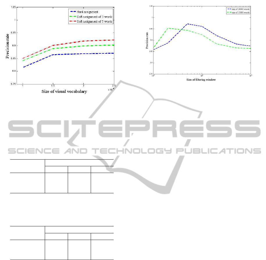
Figure 2: Comparison of the classiﬁcation precision under

different sizes of assignment window and sizes of visual vo-

cabulary.The red line represent the assignment window of 5

words, the green one shows the assignment of 3 words, and

the blue one represent the hard assignment.

Table 1: Comparison of the classiﬁcation precision under

different sizes of assignment window(1,3,5) and sizes of vi-

sual vocabulary(10000,15000,20000), in this table the σ

the assigned features is set as 5000.

Assignment

Vocabulary Size

10000 15000 20000

1 0.8142 0.8646 0.8688

3 0.8408 0.8884 0.8989

5 0.8496 0.9007 0.9184

Table 2: Comparison of the classiﬁcation precision under

different sizes of assignment window(1,3,5) and sizes of vi-

sual vocabulary(10000,15000,20000), in this table the σ

the assigned features is set as 50000.

Assignment

Vocabulary Size

10000 15000 20000

1 0.8142 0.8646 0.8688

3 0.6241 0.8391 0.8461

5 0.3169 0.4074 0.5405

5.2.2 ROC Curve

In this section, we will pass the images into the Gaus-

sian model classiﬁer under different experiment con-

straint. All of the testing images were selected from

the Oxford buildings dataset, representing some typ-

ical buildings in Oxford campus. Before the exper-

iment, we ﬁltered out the junk images, in which the

main buildings are hidden by other things or the con-

tent has nothing to do with the scenes. Here we adopt

the ROC curve to evaluate the performance of classi-

ﬁer.

As what has been shown in Figure.4, there are

some ROC curves under different scenes being listed.

In the left part, left column of the Figure.4 shows

Figure 3: Comparison of classiﬁcation precision under dif-

ferent sizes of words ﬁltering window and the visual vocab-

ulary.The blue line represent the ﬁltering window impact on

precision under vocabulary of 20000 words, and the green

one represent the size of 15000.

the ROC curve generated by the common Gaussian

model; its obvious that the common Gaussian model

may face a distinguishing ability loss on some scenes,

because of the similarity between the scene with other

ones and the insufﬁcient size of vocabulary .

And the right column of the Figure.4 shows the

ROC curve after we introduced the inconsistent fea-

ture ﬁltering stage; its clear that the AUC (Bradley,

1997) of the classiﬁer on each scene was improved.

Then we compared the precision under a different ﬁl-

ter window, in order to evaluate the impact on the

precision exerted by the inconsistent feature ﬁltering

stage. In Figure.3, we could witness that the suit-

able ﬁlter window could improve the recognition pre-

cision.But if the window was too ﬁne, it will cause

over-ﬁtting. A part of classiﬁcation result was shown

in Figure.5

6 CONCLUSIONS AND FUTURE

WORK

6.1 Conclusions

In this paper, we improved the typical k-means by in-

troduce the local approximation and the replace the

geometric center by the center data points, which

could reduce the computation , accelerate the clus-

tering process, and improve the robustness. Then We

put forward the soft-assignment that calculate the as-

signment weight on Gaussian Mixture Model, which

could reduce the error generated by the feature quanti-

zation stage. In order to model the scene, we adopt the

Gaussian scene model, which would not just represent

the stable features of a scene,but also take the uncer-

tainty into account.In addition to the above work, we

DynamicSceneRecognitionbasedonImprovedVisualVocabularyModel

563

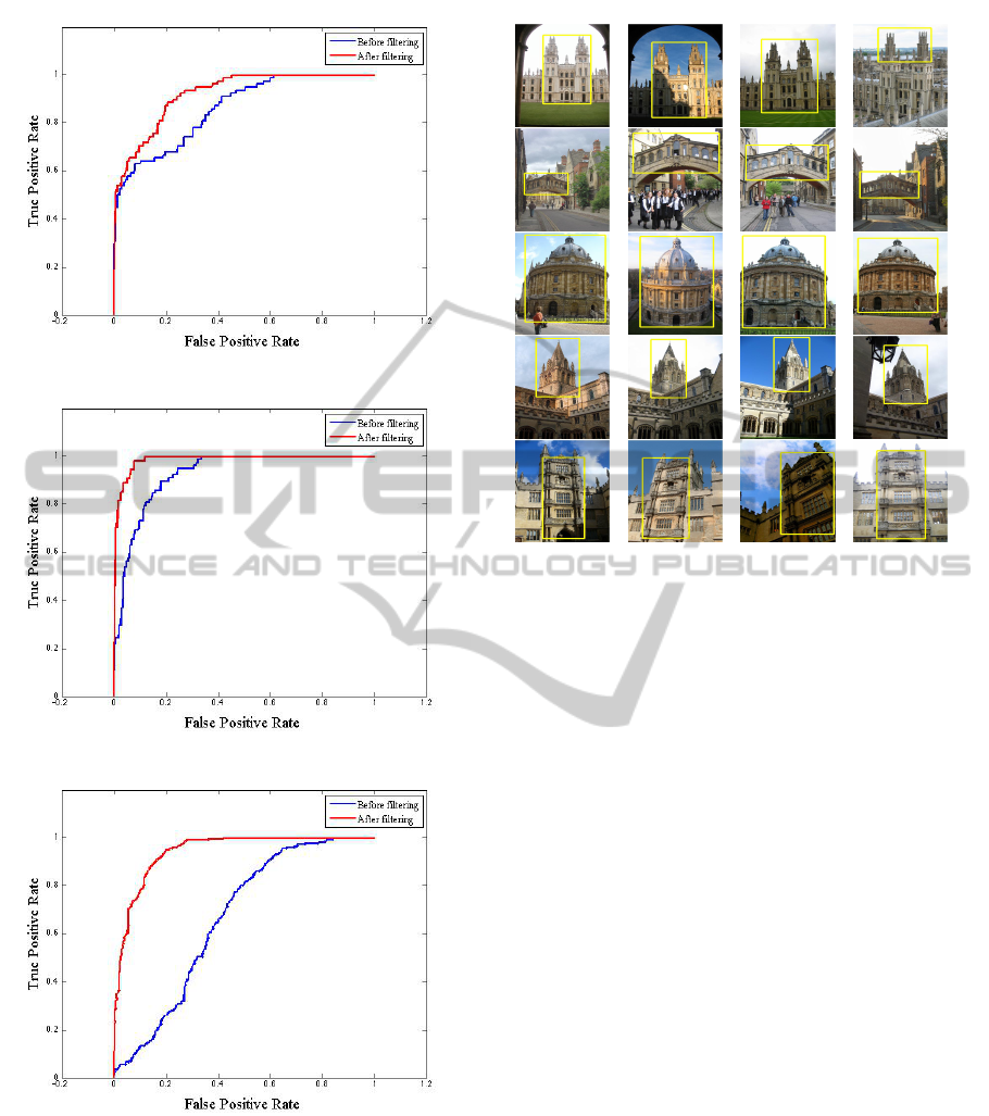
(a) scene of All Souls

(b) scene of Cornmarket

Figure 4: The ROC curve before and after the the ﬁltering

stage.By comparing the ROC curve before and after the ﬁl-

tering, it is obvious that the ﬁltering stage have improve the

performance by extend the area of AUC.This fugure shows

the ROC curve while the classiﬁer working on scenes of

All-souls, cornmarket and Radcliffe-camera.

also introduced a ﬁltering stage before the classiﬁca-

tion to improve the typical visual vocabulary scene

model by ﬁltering out the nosie features across the

Figure 5: The recognition result on some scene cate-

gories.The bounding boxes indicate the scene objects in the

images.

images of one scene, which would improve the clas-

siﬁcation performance substantially.

6.2 Future Works

For establishing a ﬂexible scene recognition system

for robot vision, we still have a lot of work to do, the

current framework relies on the statistical information

in the descriptor space but ignores the geometric in-

formation in the image. We view the method of ex-

tracting the geometric information as a necessary step

to locating the object and abstracting the high-level

features of a scene image, such as the landmarks in an

image document. In the next stage, we will concen-

trate on how to extract the local geometric informa-

tion (Johns and Yang, 2011b) and statistic informa-

tion to form the local high-level features, and how to

establish a powerful place and object recognition sys-

tem for mobile devices, which need to know not only

what is in the image but where it is.

REFERENCES

Amit, Y. and Geman, D. (1997). Shape quantization and

recognition with randomized trees. Neural computa-

tion, 9(7):1545–1588.

Bradley, A. P. (1997). The use of the area under the

VISAPP2014-InternationalConferenceonComputerVisionTheoryandApplications

564

roc curve in the evaluation of machine learning algo-

rithms. Pattern recognition, 30(7):1145–1159.

Chum, O., Philbin, J., Sivic, J., Isard, M., and Zisserman,

A. (2007). Total recall: Automatic query expansion

with a generative feature model for object retrieval. In

Computer Vision, 2007. ICCV 2007. IEEE 11th Inter-

national Conference on, pages 1–8. IEEE.

Elkan, C. (2003). Using the triangle inequality to accelerate

k-means. In ICML, volume 3, pages 147–153.

Felzenszwalb, P. F., Girshick, R. B., McAllester, D., and

Ramanan, D. (2010). Object detection with discrim-

inatively trained part-based models. Pattern Analy-

sis and Machine Intelligence, IEEE Transactions on,

32(9):1627–1645.

Johns, E. and Yang, G.-Z. (2011a). From images to

scenes: Compressing an image cluster into a single

scene model for place recognition. In Computer Vi-

sion (ICCV), 2011 IEEE International Conference on,

pages 874–881. IEEE.

Johns, E. and Yang, G.-Z. (2011b). Place recognition

and online learning in dynamic scenes with spatio-

temporal landmarks. In BMVC, pages 1–12.

Lepetit, V., Lagger, P., and Fua, P. (2005). Randomized

trees for real-time keypoint recognition. In Computer

Vision and Pattern Recognition, 2005. CVPR 2005.

IEEE Computer Society Conference on, volume 2,

pages 775–781. IEEE.

Li, F. and Kosecka, J. (2006). Probabilistic location

recognition using reduced feature set. In Robotics

and Automation, 2006. ICRA 2006. Proceedings 2006

IEEE International Conference on, pages 3405–3410.

IEEE.

Lowe, D. G. (1999). Object recognition from local scale-

invariant features. In Computer vision, 1999. The pro-

ceedings of the seventh IEEE international conference

on, volume 2, pages 1150–1157. Ieee.

Mikolajczyk, K., Leibe, B., and Schiele, B. (2006). Multi-

ple object class detection with a generative model. In

Computer Vision and Pattern Recognition, 2006 IEEE

Computer Society Conference on, volume 1, pages

26–36. IEEE.

Mikolajczyk, K. and Schmid, C. (2005). A perfor-

mance evaluation of local descriptors. Pattern Analy-

sis and Machine Intelligence, IEEE Transactions on,

27(10):1615–1630.

Mikolajczyk, K., Tuytelaars, T., Schmid, C., Zisserman, A.,

Matas, J., Schaffalitzky, F., Kadir, T., and Van Gool,

L. (2005). A comparison of afﬁne region detectors.

International journal of computer vision, 65(1-2):43–

72.

Moosmann, F., Triggs, W., and Jurie, F. (2006). Random-

ized clustering forests for building fast and discrimi-

native visual vocabularies.

Narzt, W., Pomberger, G., Ferscha, A., Kolb, D., M

uller, R.,

Wieghardt, J., H

ortner, H., and Lindinger, C. (2006).

Augmented reality navigation systems. Universal Ac-

cess in the Information Society, 4(3):177–187.

Philbin, J., Chum, O., Isard, M., Sivic, J., and Zisserman, A.

(2007a). Object retrieval with large vocabularies and

fast spatial matching. In Computer Vision and Pat-

tern Recognition, 2007. CVPR’07. IEEE Conference

on, pages 1–8. IEEE.

Philbin, J., Chum, O., Isard, M., Sivic, J., and Zisserman, A.

(2007b). Object retrieval with large vocabularies and

fast spatial matching. In Computer Vision and Pat-

tern Recognition, 2007. CVPR’07. IEEE Conference

on, pages 1–8. IEEE.

Philbin, J., Chum, O., Isard, M., Sivic, J., and Zisserman,

A. (2008). Lost in quantization: Improving partic-

ular object retrieval in large scale image databases.

In Computer Vision and Pattern Recognition, 2008.

CVPR 2008. IEEE Conference on, pages 1–8. IEEE.

Sivic, J. and Zisserman, A. (2003). Video google: A text

retrieval approach to object matching in videos. In

Computer Vision, 2003. Proceedings. Ninth IEEE In-

ternational Conference on, pages 1470–1477. IEEE.

DynamicSceneRecognitionbasedonImprovedVisualVocabularyModel

565