2D-3D Face Recognition via Restricted Boltzmann Machines
Xiaolong Wang
1
, Vincent Ly
1
, Rui Guo
2
and Chandra Kambhamettu
1
1
University of Delaware, Newark, DE, U.S.A.
2
The University of Tennessee, Knoxville, U.S.A.
Keywords:
Restricted Boltzmann Machines, Canonical Correlation Analysis, Heterogeneous Face Recognition, Match-
ing, Feature Extraction.
Abstract:
This paper proposes a new scheme for the 2D-3D face recognition problem. Our proposed framework mainly
consists of Restricted Boltzmann Machines (RBMs) and a correlation learning model. In the framework,
a single-layer network based on RBMs is adopted to extract latent features over two different modalities.
Furthermore, the latent hidden layer features of different models are projected to formulate a shared space
based on correlation learning. Then several different correlation learning schemes are evaluated against the
proposed scheme. We evaluate the advocated approach on a popular face dataset-FRGCV2.0. Experimental
results demonstrate that the latent features extracted using RBMs are effective in improving the performance
of correlation mapping for 2D-3D face recognition.
1 INTRODUCTION
Over the past few years, face recognition remains one
of the most popular topics in machine learning and
computer vision. Application based on face recogni-
tion technology (FRT) has been widely used in many
areas such as security and multimedia. However, the
recognition performance still degrades when affected
by factors, such as illumination, pose and expression.
To alleviate these influences, some researchers try to
conduct face recognition via other modalities, such as
Near-infrared (NIR) and 3D. 3D data, especially, has
been widely used in face recognition. Recently, facil-
itated by the emerging low cost 3D sensing devices,
such as Microsoft Kinect, Asus Xtion PRO, a large
variety of RGB-Depth sensing techniques have been
deployed to biometric signal aggregation and process-
ing (Shotton et al., 2011). Meanwhile, 2D-3D het-
erogeneous face recognition has also attracted more
interests. Heterogeneous face recognition refers to
matching face images across different modalities.
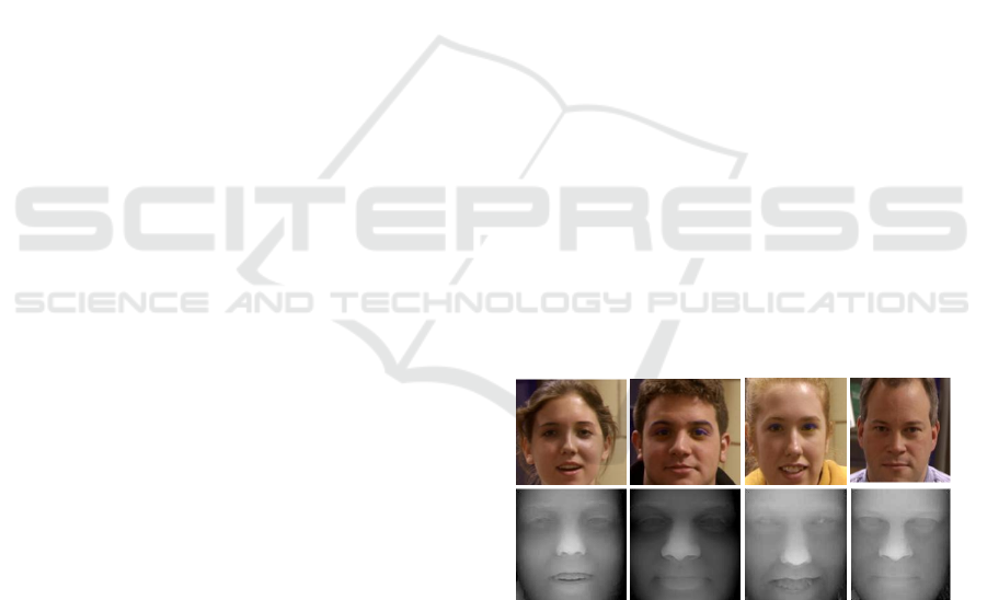
Compared with face recognition using visible im-
ages, heterogeneous face recognition is more chal-
lenging, as illustrated in Figure.1. The individual’s
identity from 2D image is difficult to be determined
using a 3D depth image. The difficulty is due to the
dissimilar appearances of the 2D face image and the
3D face image. In this work, we focus on face recog-
nition from 2D to 3D.
Compared to visible face recognition, the works
Figure 1: Examples of 2D and 3D face images. 2D faces
(first row) associated with their corresponding depth im-
age(second row).
related with heterogeneous face recognition between
2D and 3D are not widely studied. In (Rama et al.,
2006), Partial Principal Component Analysis (P
2
CA)
was used to extract features and reduce features di-
mension in the 3D and 2D data separately. Their ex-
perimental results revealed that P
2
CA could minimize
the influence of illumination. Riccio et al.(Riccio
and Dugelay, 2005) proposed to use predefined con-
trol points to calculate the geometrical invariants to
correct the pose variation for 2D/3D face recogni-
tion. Afterwards, many researchers discovered the ef-
fectiveness of Canonical correlation learning (CCA)
in this problem. Yang et al. (Yang et al., 2008)
adopted CCA to learn the mapping relation among
corresponding patches between 2D texture image and
3D depth image. The idea of utilizing CCA as the
major technique for mapping between two different
574
Wang X., Ly V., Guo R. and Kambhamettu C..
2D-3D Face Recognition via Restricted Boltzmann Machines.
DOI: 10.5220/0004736505740580
In Proceedings of the 9th International Conference on Computer Vision Theory and Applications (VISAPP-2014), pages 574-580
ISBN: 978-989-758-004-8
Copyright
c
2014 SCITEPRESS (Science and Technology Publications, Lda.)

modalities is also applied in work (Huang et al., 2012;
Wang et al., 2013).
The aim of correlation learning is to maximize the
intra-class similarity of the same individual within the
projected subspace. As we know, CCA is a stan-
dard algorithm for calculating the linear projection
of two random vectors which are maximally corre-
lated. Kernel canonical correlation analysis (KCCA)
extends CCA into nonlinear projection. KCCA per-
forms better at capturing the maximally correlated
nonlinear projection. It tries to find kernel Hilbert
spaces with kernel functions. CCA and KCCA are
adopted in learning features of multiple modalities,
then can be used in fusion for classification (Sargin
et al., 2007); especially under the situation when two
modalities are used in the training phase and only one
modality is available in the prediction phase. There
are lots of applications across many different areas,
such as natural language analysis (Vinokourov et al.,
2002; Dhillon et al., 2011), age estimation (Guo and
Wang, 2012), signal processing across multimodals
(Slaney and Covell, 2000). The success of aforemen-
tioned works sheds the light in the research of het-
erogeneous 2D/3D face mapping which highlights the
significance of correlation learning.
Recently, RBM is found to be effective in learn-
ing correlation among multi-modalities (Ngiam et al.,
2011; Srivastava and Salakhutdinov, 2012). As a
member of the Boltzamnn Machine family, RBM at-
tracts a resurgent study interest by inheriting the ex-
cellent ability of representation learning in an iterative
way. Through the weights and offset parameters ad-
justing, the bipartite structured net efficiently learns
the nested abstractions from the raw data from high
dimension space. RBM benefits itself in terms of the
hierarchical feature extraction ability and the unsu-
pervised training manner. Facilitated by these merits,
RBM is found to be effective. As we know, for cross
modality learning, data from two different modalities
is only available during the training phase. During
the testing phase, only the data from a single modal-
ity is available. Therefore, learning an efficient single
modality feature has become one essential step in this
matching work. In (Ngiam et al., 2011), Ngiam et
al. demonstrated that an auxiliary non-linear network
can capture the relationship among different modali-
ties. Motivated by their work, we plan to explore the
feasibility of feature learning using single-layer net-
work in 2D/3D face recognition.
There are several novelties in our work. First, a
single-layer network is introduced to deal with the
face recognition problem between 2D and 3D cou-
pled with correlation mapping. Based on our knowl-
edge, this is the first time that RBM model has been
adopted in heterogeneous face recognition. The pro-
posed method offers better performance relative to the
existing correlation learning schemes. This scheme
can also be adopted in other related heterogeneous
recognition works. The experimental results demon-
strate the effectiveness of our scheme compared with
reliance only on the correlation learning scheme. Sec-
ond, to measure the generality of this scheme, differ-
ent correlation methods have been compared for ef-
ficiency along with the layer features (2D RBM and
3D RBM features). In addition, the matching perfor-
mance between two different modalities of different
facial parts has been analyzed.
The rest of the paper is structured as follows. In
Section 2, we introduce the proposed scheme. Exper-
imental results are discussed in Section 3, and Section
4 provides conclusions.
2 OUR APPROACH
In this section, we describe our approach for the
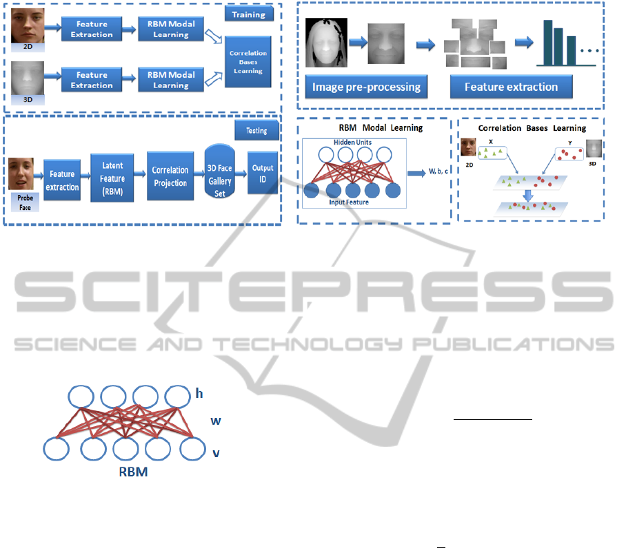
task of 2D-3D face recognition. Figure 2 shows an
overview of our scheme. After pre-processing and
extracting the feature from the images, RBM is con-
ducted. Then correlation learning is performed to
learn the projection matrix within each region be-
tween the two modalities. This will help project fea-
tures of different modalities into a shared represen-
tation space. In general, our scheme mainly includes
four parts, which are raw feature extraction (including
image pre-processing), latent feature extraction(using
RBM), correlation learning and matching. In the fol-
lowing paragraph, we will introduce the main algo-
rithms used in each part.
2.1 Restricted Boltzmann Machines
Recently, deep learning has been widely used in ma-
chine learning and computer vision. One of the fa-
mous works is trying to examine how deep sigmoidal
networks can help obtain better representation for
handwritten classification (Hinton and Salakhutdinov,
2006). The key part is to conduct multi-layer training
based on Restricted Boltzmann Machines(RBMs).
This scheme achieved excellent classification results
on this sort of problems.
RBM belongs to the category of Markov Random
Field. Compared with Boltzmann Machines (BMS),
RBMs further restrict BMs to the connection between
visible-visible layer and hidden-hidden connections
(within the intra-layers). An RBM bipartite structure
can be illustrated as in Figure 3, where w is the weight
connecting the hidden layers(h) and visible layers(v).
2D-3DFaceRecognitionviaRestrictedBoltzmannMachines
575
(a) (b)
Figure 2: The proposed framework for 2D-3D face recognition.(a) Illustration of training and testing scheme. During the
training phase, corresponding 2D and 3D face images of the same individual are used to learn RBM model and correlation
basis. During the testing phase, we firstly extract 2D probe image feature. Then after hidden latent feature extraction and
correlation projection, the probe images will be matched against the gallery set to get the corresponding ID. (b) Illustration
of principal components of the proposed scheme. For the Pre-processing section, all the images (2D/3D) are cropped to the
same size. The pre-processing of 3D images also include image denoising and hole filling. In our work, face is first divided
into eleven facial parts, then feature extraction and RBM model learning is conducted within each part. The output latent 2D
and 3D features acquired from RBM model are used to learn the basis of correlation learning model.
Figure 3: Illustration of RBM structure, where h indicates
the hidden unit and v indicates visible unit. w is the weight
connecting v and h.
From the model illustrated in Figure 3, we find that
RBM is not a direct graphical model comprised of
hidden variables(h) and visible variables(v). In ad-
dition, there is no connection between the variables
of the same layer (e.g. within visible or hidden layer).
The energy function E(v,h) of an RBM is formulated
as:
E(v, h) = −
∑
i
b
i
v
i
−
∑
j
c
j
h
j
−
∑
i, j
W
i j
v
i
h
j
(1)
where W
i j
represents the weight between the visible
layer unit i and hidden layer unit j. The parameters
c and b indicate the basis of hidden and visible layers
respectively. The parameters W
i j
, c and b can be es-
timated using maximum likelihood parameter estima-
tion (Hinton and Salakhutdinov, 2006). This scheme
can help minimize the energy states drawn from the
data distribution and raise the energy states which are
improbable given the data (Bengio, 2009). The join
probability distribution is calculated as
P(v, h) =
exp(−E(v, h))
Z
(2)
where Z =
∑
v,h
exp(−E(v, h)) indicates the Boltz-
mann partition function. We can also calculate the
marginal distribution of the visible units by summing
up the possible hidden units, which can be calculated
as
P(v) =
1
Z
∑
h
exp(−E(v, h))
(3)
With regard to the RBM structure listed in Figure 3,
the units in visible and hidden layers are conditionally
independent. When the units are binary, which means
v, h ∈ [0, 1], the probabilistic version of the neuron ac-
tivation can be represented as:
P(v
i
= 1|h) = sigm(b
j
+W
0
j
h)
P(h
j
= 1|v) = sigm(c
i
+W
i
v)
(4)
Compared with the binary input values, real val-
ued data can be well modeled using Gaussian
RBM(GRBM) (Hinton and Salakhutdinov, 2006).
GRBM does a good job at modeling continuous mul-
tivariate data. There are many applications using
GRBM, including action recognition (Wang et al.,
2011), speech recognition (Mohamed et al., 2012),
etc. In general, GRBM can be regarded as a mixture
of diagonal Gaussians with shared W , c and b param-
VISAPP2014-InternationalConferenceonComputerVisionTheoryandApplications
576

eters. Its energy function is defined as follows:
E
0
(v, h) = −
1
2
∑
i
(v
i
− b
i
)
2
σ
2
i
−
∑
i, j
W
i j
v
i
h
j
−
∑
j
c
j
h
j
(5)
Under this model, the conditional distributions for
inference and generation are calculated as follows:
P(v
i
|h) = N(b
i
+ σ
2
i
∑
j
W
i j
h
j
,σ
2
i
))
P(h
j
= 1|v) = sigm(c
j
+
∑
i
W
i j
v
i
)
(6)
where N(·) denotes the Gaussian density, and sigm is
the logistic function. In our work, GRBM is applied
to learn the single data representation.
2.2 CCA
Canonical correlation analysis(CCA) (Sutton and
Barto, 1998) has been widely used in multivari-
ate analysis. It was first advocated by Hotelling
(Hotelling, 1936) to calculate the basis vectors for two
related multidimensional variables and can be used
to maximize the correlation between these two sets
of related variables. CCA methods have been widely
used in machine learning and computer vision prob-
lems, such as action recognition(Kim et al., 2007),
face recognition(Li et al., 2009). After projecting the
data to high-dimensional space, CCA can be modeled
as the relation between these two sets of variables.
Suppose (x, y) is the corresponding data set. It in-
cludes N pairs of samples x
i
, y
i
. CCA is used to learn
the projection matrix w
x
and w
y
to maximize the cor-
relation between the projected matrix w
T
x
x and w
T
y
y.
That is to maximize the following correlation equa-
tion:
v =
w
T
x
C
xy
w
y
q
w
T
x
C
xx
w
x
w
T
y
C
yy
w
y
(7)
where C
xx
and C
yy
indicate the intra-class con-
variance matrices. v is the correlation coefficient.
And C
xy
and C
yx
indicate the inter-class con-variance
matrices. Because v is invariant to the scaling of w
x
and w
y
, CCA optimization problem can be equivalent
to maximizing w
T
x
C
XY
w
y
. This subjects to w
T
x
C
xx
w
x
=
1 and w
T
y
C
yy
w
y
= 1. (Hardoon et al., 2004) shows w
x
can be solved by using the following eigenvalue prob-
lem,
C
xy
C
−1
yy
C
yx
w
x
= λ
2
C
xx
w
x
(8)
where λ is the eigenvalue associated with the eigen-
vector w
x
. To stabilize the solution, regularization
terms r
x
and r
y
are always added to each data set
(Hardoon et al., 2004). Then v becomes
v =
w
T
x
C
xy
w
y
q
w
T
x
(C
xx
+ λI)w
x
w
T
y
(C
yy+
λI)w
y
(9)
Experiment results prove that Regularized
CCA(rCCA) performs better than CCA in our
work.
2.3 Kernel CCA
Because of its linearity, CCA may not be a good
solver when dealing with some nonlinear correla-
tion problems (Hardoon et al., 2004). Kernel CCA
(KCCA) performs better than CCA in finding nonlin-
ear projection of the two views (Hardoon et al., 2004).
The main idea of KCCA is to project the data into
a higher-dimension feature space using kernel func-
tions. In this paper, we use the Gaussian kernel as the
kernel function of KCCA, which can be represented
as
k(x, y) = e
−
||x−y||
2σ
2
(10)
Then the direction of w
x
and w
y
can be represented
as the data onto the direction α and β, which are
w
x
= Xα and w
y
= Y β. Let M
x
= X
T
X and M
y
= Y
T
Y
be kernel matrices corresponding to the two represen-
tation. Then v can be represented as
v =
α
T
M
x
M
y
β
q
α
T
M
2
x
α β
T
M
2
y
β
(11)
To force non-trivial learning on the correlation by
dealing with the overfitting and finding irrelevant cor-
relations, a regularization is always applied to KCCA.
Correlation coefficient v becomes
v =
α
T
M
x
M
y
β
q
(α
T
M
2
x
α + ka
T
M
x
α)(β
T
M
2
y
β + kβ
T
M
y
β)
(12)
Then the generalized eigenvalue problem becomes
(M
x
+ kI)
−1
M
y
(M
y
+ kI)
−1
M
x
α = λ
2
α
(13)
Where λ is the eigenvalue corresponding to the eigen-
vector w
x
. Then the whole equation becomes the stan-
dard eigenproblem Ax = λx. In our experiments, k
is set to 0.01. If k = 0, then it becomes the standard
KCCA. In our work, regularization is found to be use-
ful.
2D-3DFaceRecognitionviaRestrictedBoltzmannMachines
577
3 EXPERIMENT
In this section, we demonstrate the dataset used in this
work. We also describe the details of our experiment
methodology as well as the analysis of experiment re-
sults.
3.1 Dataset
To evaluate our proposed scheme, we use FRGCv2.0
database (Phillips et al., 2005). The images within
the dataset include pose, expression and illumination
changes, which is as illustrated in Figure 1. We ran-
domly choose 300 subjects from FRGCv2.0. For each
subject, two visible texture images and two corre-
sponding 3D range images are selected. The whole
database is divided into two parts, training set and
testing set. The training set contains the 2D-3D pairs
of 225 subjects, and the testing set includes other 75
subjects. Note that in all of our experiments, there is
no overlap between the training and testing data. This
means the images of the same individual are never
used in the training and testing phase at the same time.
Figure 4: Illustration of face parts division. To be concise,
only 2D face image is used. 3D face images also follow the
same division scheme.
3.2 Pre-processing
To get the depth image, we follow the procedure in
(Xu et al., 2009). The main problem for obtaining
the depth image from 3D point cloud is the noise re-
moval and hole filling. To reduce the noise, we apply
the mean value filter with the kernel size 5 × 5 cen-
tered with evaluating pixel. If the absolute difference
between the central pixel and mean value is greater
than our predefined threshold, then this pixel will be
regarded as an outlier and replaced. Linear interpo-
lation based on the neighboring pixels is applied to
calculate the value of the center pixel value and used
to fill the hole.
Before conducting the experiments, all 2D and
3D images are aligned and cropped to the same size,
128 × 128 pixels, based on eyes coordinates. Since
there are many variations (expression, pose), instead
of using the whole face (Huang et al., 2010), we use
facial parts. The regions of our face parts are illus-
trated in Figure 4. Different from (Yang et al., 2008),
the parts used in our experiment have semantic mean-
ing, e.g. eyebrow, eyes, nose, mouth, cheeks and
etc. Because there are pose and expression changes
in FRGCv2.0, we adopt the method for face division
in (Kumar et al., 2009). Each extracted face part is
enlarged to alleviate the influence brought by these
factors. The division of the face is illustrated in Fig-
ure 4.
3.3 Learning Scheme and Matching
Pixel intensity is used as the feature in this work. Let
us assume the 2D/3D feature pairs in each face part
are given as (F
2d
, F
3d
). Then PCA whitening is ap-
plied to the feature pairs separately. The output fea-
ture pairs are noted as (F
0
2d
, F
0
3d
). In our work, we
set 24 as the dimension of PCA whitening. Fea-
ture mean value normalization is also applied. Then
GRBM is used to get the representation of (F
0
2d
, F
0
3d
)
separately. The hidden layer variables extracted using
GRBM model are (F
h
2d
, F
h
3d
). After correlation learn-
ing, we can obtain two projection directions W
2d
and
W
3d
. (F
h
2d
, F
h
3d
) are projected into the shared subspace
using x = w
T
x
F
h
2d
and y = w
T
y
F
h
3d
. w
x
and w
y
are ob-
tained during the training process. Then the similarity
score s(x, y) can be obtained using the following nor-
malized score function:
s(x, y) =
x · y
(||x|| · ||y||)
(14)
Figure 5: A bar plot of matching accuracy of different fa-
cial parts. The number listed here corresponds to the face
part number in Fig 4. The results listed here are based on
GRBM+rKCCA scheme.
3.4 Experiment Results and Analysis
As described above, we want to investigate the perfor-
mance of different facial parts for 2D/3D face recog-
nition. As far as we know, this is the first time that the
effectiveness of different face parts for 2D-3D face
recognition has been evaluated.
VISAPP2014-InternationalConferenceonComputerVisionTheoryandApplications
578
Table 1: Assignment of weight for each facial part. The number is the same as illustrated in Fig.4.
Face Part # 1 2 3 4 5 6 7 8 9 10 11
w
t
0.25 0.25 0.25 0.30 0.30 0.50 0.35 0.15 0.15 0.10 0.10
Figure 6: A bar plot of matching accuracy of different algo-
rithms.
Table 2: Performance of different schemes comparison.
Model Accuracy
CCA 0.911
rCCA 0.924
rKCCA 0.931
GRBM+rCCA 0.952
GRBM+rKCCA 0.960
From our experimental results listed in Figure 5,
we find that there is a significant difference among
face parts for face recognition. The facial part near
the nose region plays the most important role in the
matching scheme. Considering the different match-
ing accuracy of each part, the weighed sum rule (Jain
et al., 2011) is used as the fusion tool to obtain the
final result. Weighted sum rule can be represented as
F =
n
∑
t=1
w
t
s
t
,
(15)
where F is the matching score and n is the total num-
ber of face parts. w
t
is the weight value corresponding
to the matching score s
t
of face part t. The assignment
of value w
t
for each facial part is illustrated in Table
1. The matching results after different face parts fu-
sion are shown in Table 2. A better matching result is
obtained after fusion of different face parts. From the
results listed in Figure 6, we find that RBM can boost
the performance of correlation mapping.
In this paper, we also evaluate the proposed algo-
rithm using the global face. The accuracy is 55.0%
(based on GRBM+rKCCA). This result also demon-
strates that the single global face mapping between
2D and 3D face data is not appropriate for describ-
ing the relationship between 2D and 3D face data.
Since the correspondence of different face parts be-
tween 2D and 3D is not identical, it’s not accurate to
use the whole face for correlation learning between
two modalities.
4 CONCLUSIONS
In this paper, one single-layer network was proposed
for heterogeneous 2D/3D face recognition problem.
Our experiment results proved that learning correla-
tion representation on the layer features extracted us-
ing RBM resulted in a better matching performance.
Meanwhile, we also explored the effectiveness of dif-
ferent facial parts in 2D/3D face matching. The re-
sults indicated that fusion with different facial parts
can achieve a significant improvement compared with
the global face.
The proposed scheme is an excellent addition to
the corpus of heterogeneous face recognition works.
The proposed learning scheme can also be adopted
by other 2D/3D face recognition works as the major
learning scheme.
REFERENCES
Bengio, Y. (2009). Learning deep architectures for ai. Foun-
dations and trends
R
in Machine Learning, 2(1):1–
127.
Dhillon, P., Foster, D. P., and Ungar, L. H. (2011). Multi-
view learning of word embeddings via cca. In Ad-
vances in Neural Information Processing Systems,
pages 199–207.
Guo, G. and Wang, X. (2012). A study on human age esti-
mation under facial expression changes. In Computer
Vision and Pattern Recognition (CVPR), 2012 IEEE
Conference on, pages 2547–2553. IEEE.
Hardoon, D. R., Szedmak, S., and Shawe-Taylor, J. (2004).
Canonical correlation analysis: An overview with ap-
plication to learning methods. Neural Computation,
16(12):2639–2664.
Hinton, G. E. and Salakhutdinov, R. R. (2006). Reducing
the dimensionality of data with neural networks. Sci-
ence, 313(5786):504–507.
Hotelling, H. (1936). Relations between two sets of vari-
ates. Biometrika, 28(3/4):321–377.
Huang, D., Ardabilian, M., Wang, Y., and Chen, L. (2010).
Automatic asymmetric 3d-2d face recognition. In
Pattern Recognition (ICPR), 2010 20th International
Conference on, pages 1225–1228. IEEE.
2D-3DFaceRecognitionviaRestrictedBoltzmannMachines
579

Huang, D., Ardabilian, M., Wang, Y., and Chen, L. (2012).
Oriented gradient maps based automatic asymmetric
3d-2d face recognition. In Biometrics (ICB), 2012 5th
IAPR International Conference on, pages 125–131.
IEEE.
Jain, A. K., Ross, A. A. A., and Nandakumar, K. (2011).
Introduction to biometrics. Springer.
Kim, T.-K., Wong, S.-F., and Cipolla, R. (2007). Tensor
canonical correlation analysis for action classification.
In Computer Vision and Pattern Recognition, 2007.
CVPR’07. IEEE Conference on, pages 1–8. IEEE.
Kumar, N., Berg, A. C., Belhumeur, P. N., and Nayar, S. K.
(2009). Attribute and simile classifiers for face verifi-
cation. In Computer Vision, 2009 IEEE 12th Interna-
tional Conference on, pages 365–372. IEEE.
Li, A., Shan, S., Chen, X., and Gao, W. (2009). Maxi-
mizing intra-individual correlations for face recogni-
tion across pose differences. In Computer Vision and
Pattern Recognition, 2009. CVPR 2009. IEEE Confer-
ence on, pages 605–611. IEEE.
Mohamed, A.-r., Dahl, G. E., and Hinton, G. (2012).
Acoustic modeling using deep belief networks. Audio,
Speech, and Language Processing, IEEE Transactions
on, 20(1):14–22.
Ngiam, J., Khosla, A., Kim, M., Nam, J., Lee, H., and Ng,
A. (2011). Multimodal deep learning. In Proceed-
ings of the 28th International Conference on Machine
Learning (ICML-11), pages 689–696.
Phillips, P. J., Flynn, P. J., Scruggs, T., Bowyer, K. W.,
Chang, J., Hoffman, K., Marques, J., Min, J., and
Worek, W. (2005). Overview of the face recogni-
tion grand challenge. In Computer vision and pattern
recognition, 2005. CVPR 2005. IEEE computer soci-
ety conference on, volume 1, pages 947–954. IEEE.
Rama, A., Tarres, F., Onofrio, D., and Tubaro, S. (2006).
Mixed 2d-3d information for pose estimation and face
recognition. In Acoustics, Speech and Signal Pro-
cessing, 2006. ICASSP 2006 Proceedings. 2006 IEEE
International Conference on, volume 2, pages II–II.
IEEE.
Riccio, D. and Dugelay, J.-L. (2005). Asymmetric 3d/2d
processing: a novel approach for face recognition. In
Image Analysis and Processing–ICIAP 2005, pages
986–993. Springer.
Sargin, M. E., Yemez, Y., Erzin, E., and Tekalp, A. M.
(2007). Audiovisual synchronization and fusion us-
ing canonical correlation analysis. Multimedia, IEEE
Transactions on, 9(7):1396–1403.
Shotton, J., Fitzgibbon, A., Cook, M., Sharp, T., Finoc-
chio, M., Moore, R., Kipman, A., and Blake, A.
(2011). Real-time human pose recognition in parts
from single depth images. In Computer Vision and
Pattern Recognition (CVPR), 2011 IEEE Conference
on, pages 1297–1304. IEEE.
Slaney, M. and Covell, M. (2000). Facesync: A linear op-
erator for measuring synchronization of video facial
images and audio tracks. In NIPS, pages 814–820.
Srivastava, N. and Salakhutdinov, R. (2012). Multimodal
learning with deep boltzmann machines. In Advances
in Neural Information Processing Systems 25, pages
2231–2239.
Sutton, R. S. and Barto, A. G. (1998). Reinforcement learn-
ing: An introduction, volume 1. Cambridge Univ
Press.
Vinokourov, A., Cristianini, N., and Shawe-taylor, J. S.
(2002). Inferring a semantic representation of text via
cross-language correlation analysis. In Advances in
neural information processing systems, pages 1473–
1480.
Wang, H., Klaser, A., Schmid, C., and Liu, C.-L. (2011).
Action recognition by dense trajectories. In Computer
Vision and Pattern Recognition (CVPR), 2011 IEEE
Conference on, pages 3169–3176. IEEE.
Wang, X., Ly, V., Guo, G., and Kambhamettu, C. (2013). A
new approach for 2d-3d heterogeneous face recogni-
tion. In Multimedia (ISM), 2013 IEEE International
Symposium on. IEEE.
Xu, C., Li, S., Tan, T., and Quan, L. (2009). Automatic 3d
face recognition from depth and intensity gabor fea-
tures. Pattern Recognition, 42(9):1895–1905.
Yang, W., Yi, D., Lei, Z., Sang, J., and Li, S. Z. (2008).
2d–3d face matching using cca. In Automatic Face &
Gesture Recognition, 2008. FG’08. 8th IEEE Interna-
tional Conference on, pages 1–6. IEEE.
VISAPP2014-InternationalConferenceonComputerVisionTheoryandApplications
580
