Generalized Preemptive RANSAC

Making Preemptive RANSAC Feasible even in Low Resources Devices

Severino Gomes-Neto

1,2

and Bruno M. Carvalho

Escola Agr

ıcola de Jundia

ı, UFRN, RN 160 - Km 03, Distrito de Jundia

ı, Maca

ıba/RN, Brazil

Departamento de Inform

atica e Matem

atica Aplicada, UFRN, Campus Universit

ario Lagoa Nova, Natal/RN, Brazil

Keywords:

Preemptive RANSAC, Generalized Preemptive RANSAC, Preemption Function, BRUMA, Computer Vision.

Abstract:

This paper examines a generalized version of Preemptive RANSAC for visual motion estimation. The ap-

proach described employs the BRUMA function for dealing with varying block sizes and the percentages

of hypotheses to be removed during the hypotheses rejection phase. The generation of a ﬂexible number of

hypotheses is also performed in order to balance the preemption scheme. Experiments were performed for

both forward and side-wise motions in synthetic environment by using simulation and the ground-truth used

to compare the Standard Preemptive RANSAC and its generalized version. Simulations conﬁrmed that the

quality of the results produced by the Standard Preemptive RANSAC degrade as the hardware resources used

are decreased, as opposed to the results produced by the Generalized Preemptive RANSAC, with the results

of the Standard Preemptive RANSAC having errors up to eleven times larger than the Generalized Preemptive

RANSAC.

1 INTRODUCTION

The tasks carried in automated motion estimation are

computationally expensive, resulting in a consider-

able amount of time dedicated to perform them. Thus,

one should concentrate in achieving accurate estima-

tions in a not prohibitive amount of time when plan-

ning a computer vision system. In other words, one

needs to reach the balance between these goals in or-

der to design a good system.

We are particularly interested in the research that

focus on accelerating the methods in order to promote

their feasibility in low power and/or low cost hard-

ware setups, allowing these setups to be employed

in ﬁelds such as robotics, autonomous navigation and

several other applied Computer Vision (CV) tasks.

Computer Vision systems have made large use of

the RANSAC algorithm (Fischler and Bolles, 1981)

in order to deal with the hypothesize-and-verify prob-

lem. However, Nist

er discussed that the standard

RANSAC is not designed for executions under time

constraints (Nist

er, 2003).

The standard RANSAC ﬁrst generates hypotheses

from subsets of observations and then evaluates these

hypotheses against all the available observations in or-

der to determine which hypothesis is the best repre-

sentative of the entire population (the closest from the

ideal solution), and keeps working until it reaches a

conﬁdence threshold. This conceptual simplicity and

the results achieved made RANSAC a standard in the

CV and 3D Reconstruction (3DR) ﬁelds.

Nevertheless, the standard algorithm has insufﬁ-

cient performance in some cases. Thus, several meth-

ods were published targeting the goal of speeding up

RANSAC tasks and dealing with the trade-off be-

tween quality and time by working in three major

points: alternative hypothesize-and-verify methods,

improvements on the hypotheses generation and im-

provements on the hypotheses evaluation.

The ﬁrst approach has a variety of works, such as

MLESAC (Torr and Zisserman, 2000), AMLESAC

(Konouchine et al., 2005), KALMANSAC (Vedaldi

et al., 2005), PROSAC (Chum and Matas, 2005),

GASAC (Rodehorst and Hellwich, 2006) and GOOD-

SAC (Michaelsen et al., 2006). All of them execute

hypothesize-and-verify tasks but each one has its own

particularities, leading to algorithms that are efﬁcient

for speciﬁc classes of applications.

Nist

er’s Efﬁcient Five-Point Algorithms (Nist

er,

2004) and hypotheses generation using Graphics Pro-

cessor Units (GPUs) are examples of the second

branch that consists of speeding up the hypotheses

generation process or enhancing their quality in order

to decrease the number of generation rounds. How-

406

Gomes-Neto S. and M. Carvalho B..

Generalized Preemptive RANSAC - Making Preemptive RANSAC Feasible even in Low Resources Devices.

DOI: 10.5220/0004737004060415

In Proceedings of the 9th International Conference on Computer Vision Theory and Applications (VISAPP-2014), pages 406-415

ISBN: 978-989-758-009-3

 2014 SCITEPRESS (Science and Technology Publications, Lda.)

ever, it has been shown that each hypotheses gen-

eration method ﬁts better to certain camera motions

(

Segvi

c et al., 2007b), i.e., we do not have a single

best hypotheses generation method.

The last approach focuses on accelerating the

evaluation process or, alternatively, detecting a condi-

tion that avoids unnecessary exhaustive veriﬁcation.

This anticipation in the end task is often called pre-

emption and it is the way we choose for improving

the performance of the hypothesize-and-verify algo-

rithm (RANSAC in our work).

The need for time constraints comes from the re-

quirement of working in a range of time variability

as narrow as possible. The time constraints assure

the control over variability, but is unable to assure the

preservation of estimation accuracy by itself.

We use the Nist

er’s Preemptive RANSAC (Nist

er,

2003) (referred in the rest of the paper as P-RANSAC)

as the representative of the last mentioned approach

since it is the most used method after ten years of its

publication.

The P-RANSAC is aware of the need of chang-

ing evaluation process in order to deliver estimations

that still are in a level of accuracy compatible with

vision applications. The results presented in (Nist

er,

2003) made clear that it is possible to reach the bal-

ance between accuracy and speed of execution to de-

velop useful applications. The P-RANSAC employs

a function in order to identify the moment of preemp-

tion. This concept is simple and powerful, but the

function deﬁned in Nist

er’s work is very dependent

on number of hypotheses and observations to work

properly.

Afterwards, Nist

er speeded up the hypotheses

generation, the most costly operation in the estima-

tion process, by using the efﬁcient 5-point algorithm

(Nist

er, 2004).

Even demonstrating that the balance is possible,

Nist

er’s works are not ﬁt for every vision applica-

tion as has been pointed out in (Raguram et al., 2008;

Chum and Matas, 2008; Gomes-Neto and Carvalho,

2010). Despite the issues concerning the fact that P-

RANSAC been derived from RANSAC and conse-

quently inherits some of its limitations, the problem

that is embedded in its conception is the presence of

constant parameters that were chosen empirically or

arbitrarily.

Empirical parameters depend on the hardware

where the experiments were performed. Thus, we

have a problem to reproduce the empirical parame-

ters or to ﬁt it to distinct hardware setups. In the case

of the arbitrary parameters, one makes assumptions

that should be valid for all possible setups, and, in

the case of being wrong, that results in a bad problem

modeling. In order to circumvent that, we employ the

function BRUMA (Block Resizing for UnderManned

Amount of Assays Avoidance) (Gomes-Neto and Car-

valho, 2010), that performs a generalization of pre-

emption functions and allows parameter variations.

The idea is that when this preemption function is used

with P-RANSAC, one can achieve the balance be-

tween accuracy and time consumption by chosen pa-

rameters that ﬁt to particular hardware setups in what

we call Generalized Preemptive RANSAC (GPR).

This work presents the results of experiments by

using GPR to determine parameters that ﬁt distinct

hardware setups in order to prove the feasibility of

adapting the original P-RANSAC to running in low

resource devices.

The rest of this work is organized as follows. Sec-

tion 2 presents the Generalized Preemptive RANSAC,

while Section 3 describes the methodology employed

in the experiments. Sections 4 and 5 present the ex-

perimental results and the discussion about them, re-

spectively. Finally, Section 6 summarizes the paper,

highlighting contributions and further work.

2 GENERALIZED PREEMPTIVE

RANSAC

We now present the Generalized Preemptive

RANSAC (GPR), a framework that uses the BRUMA

function in the P-RANSAC, but also allowing the

variation of an additional parameter of the pre-

emption scheme in order to show that one ﬁxed

parameter set for all cases may not be able to balance

the preemption and control the error level of the

estimation task.

The ﬁrst goal is to produce similar results when

comparing with P-RANSAC under the same time

constraints, but selecting distinct parameters to prove

the aforementioned claim in a fair comparison stan-

dard. The second goal is to employ the GPR frame-

work in restrictive conditions, where P-RANSAC’s

estimation quality is expected to degenerate due to

lack of resources for supporting the original param-

eters selection, and show that GPR is more robust

under the same conditions, a result obtained by just

selecting the parameters in accordance with the hard-

ware limitations.

The GPR makes use of three parameters that to-

gether can control the preemptive evaluation: the

number of generated hypotheses, the size of the block

of observations that rule the hypotheses elimination

task and the fraction of hypotheses to remove in each

rejection round.

GeneralizedPreemptiveRANSAC-MakingPreemptiveRANSACFeasibleeveninLowResourcesDevices

407

The P-RANSAC preemption function (1) is given

f (i) = bM · 2

−b

c, (1)

where b.c denotes the ﬂoor operator, M is the number

of available hypotheses and B denotes a ﬁxed block

size (i.e. the amount of observations the algorithm

must test in an evaluation round to allow hypothe-

ses rejection). The BRUMA function can be seen as

a generalization of the P-RANSAC preemption func-

tion (1) and its given by

f (i) = bM

· p

−b

c, (2)

where M

denotes the amount of hypotheses at the i-

th evaluation step, p

is a scalar indicating the fraction

of hypotheses to eliminate on a rejection round and B

denotes the block size at the i-th evaluation step.

In both equations every time i reaches the block

size the algorithm sorts the available hypotheses ac-

cording their scores and discards a fraction of less

promising hypotheses, i.e., the hypotheses with the

lowest scores. The process is repeated until one of

the stop conditions occur, either a single hypothesis

remains and is the winner or the time budget is ex-

hausted and the hypotheses with the best score is the

winner.

The P-RANSAC deals with hybrid preemption

scheme emphasizing breadth as deﬁned in

∀o

, π

) =

∑

i=1

ρ(o

, h

i| j

), (3)

where h

i| j

denotes that the hypothesis chosen depends

on the observation, since the observations are grouped

in blocks. This means that its preemption function

prioritizes the coverage of hypotheses in the evalua-

tion process. However, since P-RANSAC deﬁnes a

rigid setup of parameters, it can degenerate to a pure

breadth-ﬁrst preemption scheme if it does not perform

at least one round of elimination before exhausts the

time budget.

The P-RANSAC’s preemption function inspired

BRUMA, with the latter allowing varying block sizes

(B) and fraction of hypotheses to remove (referred as

or FHR, from now on). By using BRUMA instead

of the original function, a system is able to adjust the

parameters and ﬁt pure depth-ﬁrst, pure breadth-ﬁrst

or a wider number of possibilities of hybrid preemp-

tion schemes as shown in (Gomes-Neto and Carvalho,

2010) and may also avoid degeneration due to the lack

of elimination rounds mentioned previously.

The usage of the BRUMA function allows us to

vary two of the control parameters, with the third

concerning the maximum number of hypotheses to

be generated (and indirectly the portion of time dedi-

cated to hypotheses generation).

In the generation step, P-RANSAC determines

a maximum number of hypotheses to be generated.

This number is ﬁxed at 500, and, one can empirically

see that it is easy to reach and pass this number when

working with relaxed time budgets and/or powerful

hardware. However, each CV application has a hard-

ware setup to ﬁt its demands and it is not rare to have

modest conﬁgurations even having restricted time re-

quirements.

Taking this into account, we hypothesized that in

lower capability devices the Maximum Number of

Hypotheses to Generate (MNHG) must be decreased,

and conﬁrmed it experimentally. That means that

each device must have its MNHG determined by its

individual capacities of generating and testing hy-

potheses. We will return to this point when describing

experiments and their results.

In order to save time in the evaluation process, P-

RANSAC deﬁnes a periodicity in which it has to per-

form hypotheses elimination. The period is deﬁned by

a number of observations the algorithm has already

tested before elimination and is called block size in

reference of the block of observations.

The determination of the block size has capital im-

portance in the process of evaluation, since it deter-

mines the moment that the less promising hypotheses

so far are eliminated. If the block size is smaller than

necessary, elimination starts earlier, possibly discard-

ing good hypotheses that just have not been tested

enough to estimate their scores accordingly. On the

other hand, if the block size is larger than required, a

considerable number of tests may be done over use-

less hypotheses or the tests may not performed in the

whole block, thus failing to reject any of the gener-

ated hypotheses and being the same as applying the

standard RANSAC with breadth scoring.

Nist

er determines experimentally that a block size

of 100 observations reaches a good balance. As we

mentioned before, one should be aware that balance

is a matter of hardware setup. Thus, we will show ex-

perimentally that different hardware setups will have

different associated optimal block sizes.

Finally, the fraction of hypotheses to be removed

in each rejection round determines the amount of hy-

potheses that will be discarded. Since the hypotheses

are scored for every evaluation step until reaching the

block size, a ﬁxed number of the hypotheses with the

lowest scores are eliminated.

The P-RANSAC adopts a rejection ratio of half of

the available hypotheses reducing rapidly the number

of hypotheses to analyze. The concept seems promis-

ing, but we decided to investigate the impact of chang-

VISAPP2014-InternationalConferenceonComputerVisionTheoryandApplications

408

ing this value, since the changes in the other parame-

ters may affect this choice.

3 METHODOLOGY

We made the option for simulating using synthetic

data in order to have a groundtruth reference to com-

pare the algorithms accordingly. The ﬁrst set of simu-

lations was planned to compare P-RANSAC and GPR

in a powerful hardware as a way to compare them

fairly and demonstrate that the original values of pa-

rameters used in P-RANSAC are not the unique pa-

rameter setup that works well with the balanced Pre-

emptive RANSAC. Thus, we did not focused in sur-

passing P-RANSAC performance, but in achieving a

set of parameters that aids us to prove such concept.

A second round of simulations were performed

using a low budget hardware in order to demonstrate

the slow decreasing of accuracy when using GPR as

opposed to the high error results produced when using

P-RANSAC.

A total of 1000 replications were simulated for

each setup. We modiﬁed the simulator developed by

Segvi

c and used in his works for performance (

Segvi

et al., 2007b) and accuracy (

Segvi

c et al., 2007a) eval-

uations. The original code

uses the library Boost

and the Oxford Active Vision Lab VW34

Table 1 presents a total of six time budgets we de-

ﬁned to evaluate, covering a number of possible time

restrictions that seems feasible for a wide range of

applications. The simulation setups were planned in

order to allow fair comparisons between P-RANSAC

and the tuned GPR. To reach this goal we ﬁxed some

simulation parameters while the experimental param-

eters have their values determined and tested in each

simulation setup.

Simulation parameters that remained ﬁxed along

all the experiments were the number of observations

(1000), the ﬁve point hypotheses generation algo-

rithm (Nist

er, 2004), (Li and Hartley, 2006), (

Segvi

et al., 2007b) and Gaussian white noise (σ = 1).

We planned to vary the number of observations,

but not signiﬁcant inﬂuence had been detected from

such variation; thus, we ﬁxed the number of obser-

vations to be equal to the number originally used in

P-RANSAC. The option for ﬁve point algorithm was

natural since it was ﬁrstly used in the P-RANSAC and

Available at http://www.zemris.fer.hr/∼ssegvic/src/

evalpose.tar.gz

Available at http://www.boost.org/

Available at http://www.doc.ic.ac.uk/∼ajd/Scene/

Release/vw34.tar.gz

Gaussian white noise was used since it is very dissem-

inated in vision systems testing when working with

synthetic data.

Table 1 presents the parameters used in the exper-

iments which were chosen to represent several appli-

cation requirements’ scenarios. We used two types

of synthetic motion (forward and side-wise) in order

to collected the Translational Error (TError) of each

algorithm in both circumstances. The motions were

not combined and TError was computed separately

by decomposing the winner hypothesis into the ro-

tation matrix and translation vector, with the vector

being used to determine the angular error concerning

the ground truth vector.

The sets of generated hypotheses were used by

both algorithms and scores were computed summing

up reprojection error of every available hypothesis for

a certain number of observations. In order to make

sure that all the hypotheses have the same number of

tests in the case of preemption by time expiration, the

error for a given observation is computed for all hy-

potheses before moving on to another observation.

We altered the hypotheses generation step to deal

with the variable MNHG and, as a consequence, we

included an extra test that prevents the generation of

extra hypotheses if it reaches the determined MNHG.

This allowed both algorithms to add the remaining

time from generation task to the one third of budget

assured by default to the evaluation step.

The experiments performed to validate and test

our method were the following:

1. Validation of the method, where we executed ex-

periments using both algorithms with the same pa-

rameters to conﬁrm that both algorithms produce

identical results.

2. Adjustment of the method, where we executed

experiments with adjusted parameters in GPR, but

using standard maximum for hypotheses genera-

tion (500).

3. Test Scenario 1, where we executed experiments

with different maximum number of hypotheses (5

× budget, given in µs) for each budget and with

adjusted GPR parameters.

4. Test Scenario 2, where we executed experiments

with different maximum number of hypotheses (5

× budget) for each budget and with adjusted GPR

parameters in a low-budget hardware.

The validation experiments conﬁrmed that using

the same parameters in both P-RANSAC and GPR

produce identical results, as it should be. The result

of experiments in the other three experiments are pre-

sented in the next section.

GeneralizedPreemptiveRANSAC-MakingPreemptiveRANSACFeasibleeveninLowResourcesDevices

409

Table 1: Time budgets and their relationships in the experimental setup (MGT stands for Maximum Generation Time and

MET stands for Maximum Evaluation Time).

Budget MGT MET MNHG

(ms) Hz (budget×0.667) (budget×0.333) (budget×5)

16.667 60 11.116889 5.550111 83.335

33.333 30 22.233111 11.099889 166.665

40 25 26.68 13.32 200

50 20 33.35 16.65 250

66.667 15 44.466889 22.200111 333.335

100 10 66.7 33.3 500

4 EXPERIMENTS

The experiments were performed according the sim-

ulation methodology described in the previous sec-

tion. The hardware used in the experiments consisted

of one powerful computer and one low-budget com-

puter for the current standards. The ﬁrst computer

is equipped with an Intel Core i7 second generation

processor running at 3.07 GHz that, despite having 8

cores, had the processes launched in a Windows 7,

single-threaded console to perform all the process-

ing. The second computer is equipped with a AMD

A6-3400M processor quad core CPU, running at 1.40

GHz, in which we also launched the processes in a

Windows 7, single-threaded console.

We made the option for using single-thread pro-

cess in order to make simple and fair comparisons.

Since only one thread is available, it is simpler to

reproduce the simulations under the same conditions

and check the performance even in distinct hardware

setups and/or architectures. This also minimizes the

possible impact of any other process that may be

started by the operating system.

As mentioned in the previous Section, four experi-

ments were performed. The ﬁrst experiment was used

only to validate the results our approach. The results

of the other three experiments are now presented in a

total of three tables. These tables include information

about time budget, GPR block size, GPR rejection

fraction, the average number of generated hypotheses,

and the average error for both GPR and P-RANSAC,

and for both forward and side-wise motions.

The Table 2 shows the results of the experiments

for both forward and side-wise motions with the orig-

inal MNHG value run on the more powerful device,

while Table 3 shows the results of the same experi-

ments but with the modiﬁed MNHG running in the

same device. Finally, Table 4 shows the results with

the modiﬁed MNHG, but when run in the low-budget

device.

5 DISCUSSION

The results show that our hypothesis is correct, i.e.,

that one can ﬁnd parameters that may balance the pre-

emption scheme and produce better results than by

using the standard values originally selected for P-

RANSAC. They also demonstrate that our assumption

about MNHG is plausible, since the TError presented

small variability in some cases and a bit wider in oth-

ers.

The results of the experiments show that when the

GPR parameters are well tuned, the variability of its

results is smaller than the P-RANSAC results. We

can also infer from the results that the GPR accuracy

was consistent in every scenario. That does not means

that GPR produced the best results in all tests, but that

its ﬂexibility allows it to be tuned so it can be used

for a particular conﬁguration of application, time con-

straints and hardware.

We plotted the average errors for the forward and

the side-wise motions for both algorithms. In Figures

1 and 2 we show the results for the more powerful ma-

chine. We did not include the results of P-RANSAC

with the modiﬁed MNHG scenario in order to pre-

serve the scale of the graph, since it reached values

around ﬁve times larger than the other ones.

Figures 3 and 4 compare the results of GPR and P-

RANSAC in the modiﬁed MNHG scenario in the low-

budget device. Actually, the results of P-RANSAC

in the modiﬁed MNHG scenario are similar for both

devices, thus, the average translational errors for the

more powerful machine that were not included in Fig-

ures 1 and 2 can be inferred from the results shown on

Figures 3 and 4.

Figure 1 conﬁrms the possibility of achieving sim-

ilar results by using GPR with different parameters

selection than of the standard setup, and that the GPR

with modiﬁed value for MNHG showed less variation

in the average error relative to the variation of time

budget.

The ﬁrst charted point of Figures 1 and 2 present

VISAPP2014-InternationalConferenceonComputerVisionTheoryandApplications

410

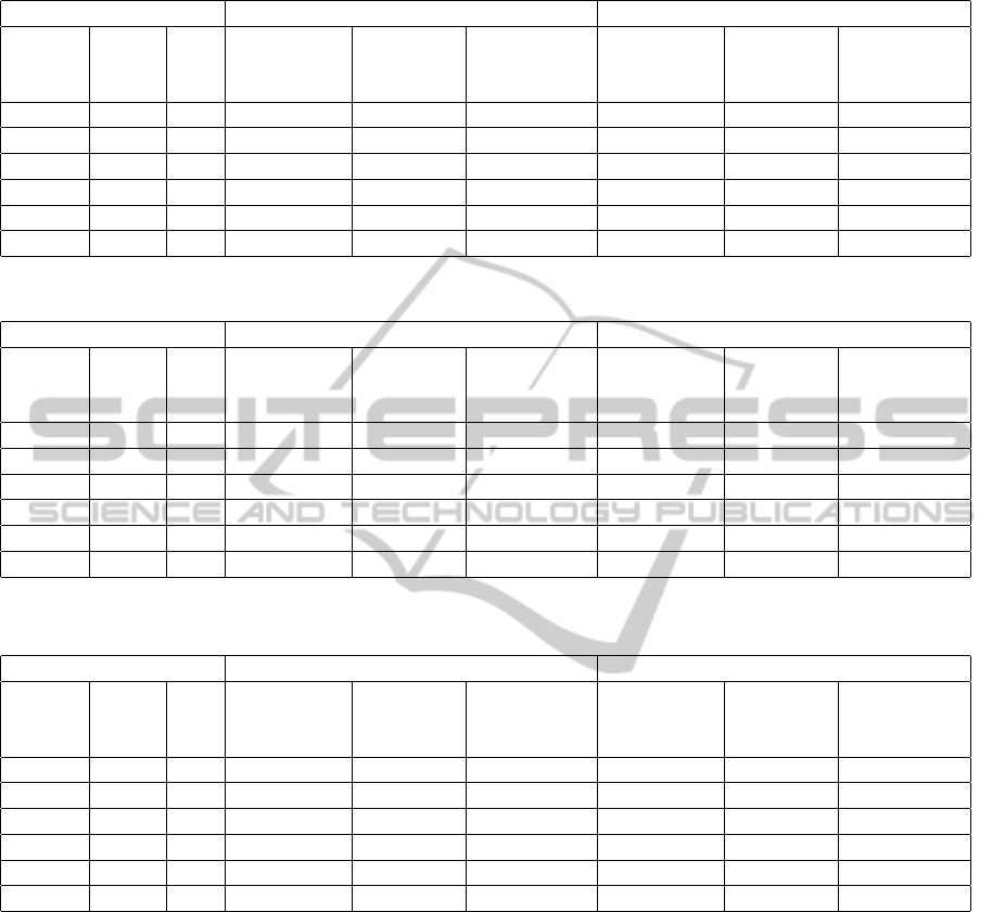
Table 2: Experiments with original value of MNHG. (FtR stands for Fraction to Remove).

Forward Motion side-wise Motion

Average Average Average Average Average Average

Budget GPR FtR Generated GPR P-RANSAC Generated GPR P-RANSAC

(ms) Block (%) Hypotheses TError (

◦

) TError (

◦

) Hypotheses TError (

◦

) TError (

◦

)

16.667 20 20 478.906 14.8458 8.31558 360.962 5.11734 5.66775

33.333 30 20 501.447 8.65899 5.94851 500.561 5.07457 4.8266

40 40 30 501.348 6.48244 6.3134 500.978 4.73236 5.08546

50 60 40 501.389 6.3561 6.15591 501.006 5.22747 4.96326

66.667 60 40 501.419 6.25041 5.92838 500.978 5.31673 4.64777

100 60 40 501.462 6.28521 16.925 501.039 5.38165 10.7852

Table 3: Experiments with modiﬁed MNHG. (FtR stands for Fraction to Remove).

Forward Motion side-wise Motion

Average Average Average Average Average Average

Budget GPR FtR Generated GPR P-RANSAC Generated GPR P-RANSAC

(ms) Block (%) Hypotheses TError (

◦

) TError (

◦

) Hypotheses TError (

◦

) TError (

◦

)

16.667 45 45 85.463 10.3403 46.6469 84.989 6.98301 55.4828

33.333 50 65 168.352 7.70724 45.871 167.978 5.95346 53.8409

40 50 65 201.395 7.36652 44.975 200.974 5.6052 53.8277

50 45 50 251.401 7.35803 42.8753 250.966 5.33252 52.456

66.667 45 50 335.423 6.67942 44.4866 334.997 4.91618 56.4664

100 45 50 501.37 6.37809 45.0267 500.984 4.79571 55.9154

Table 4: Experiments with modiﬁcation in the maximum number of hypotheses to generate, forward motion. (FtR stands for

Fraction to Remove).

Forward Motion side-wise Motion

Average Average Average Average Average Average

Budget GPR FtR Generated GPR P-RANSAC Generated GPR P-RANSAC

(ms) Block (%) Hypotheses TError (

◦

) TError (

◦

) Hypotheses TError (

◦

) TError (

◦

)

16.667 20 20 85.36 15.1992 45.763 85.029 7.51641 56.8997

33.333 30 20 168.505 11.4411 46.0835 167.963 6.11811 52.2122

40 40 40 201.454 8.08279 44.578 200.989 5.62041 56.5226

50 60 40 251.445 7.59762 44.9756 250.954 5.80402 51.546

66.667 60 40 335.426 6.79015 44.9835 334.985 5.61065 51.5363

100 60 40 501.355 6.26112 43.1999 500.959 5.29221 53.072

an isolated degenerated behavior of P-RANSAC. In a

deeper investigation, we detected that the degeneracy

is the effect of the unbalanced amount of hypotheses

and the maximum number of tests that leaded to a sce-

nario in which the algorithm discarded an insufﬁcient

amount of hypotheses to enforce the estimation qual-

ity.

Figure 2 shows a similar behavior of all three al-

gorithms, except for the GPR with standard MNHG

when the time budget is lowered for forward motion.

We also found out that the GPR with standard MNHG

was more robust for lower budgets in side-wise mo-

tion, since it did not show any signiﬁcant error in-

crease.

We have shown that one can use GPR with differ-

ent hardware conﬁgurations and constraints, in cases

where the P-RANSAC fails to produce good results.

An important detail is that the speciﬁc balance we

achieve here is related to the hardware conﬁguration

used. Different hardware conﬁgurations may, and

most certainly will, have a different set of optimal pa-

rameters.

It is necessary to mention the two main obsta-

cles for tuning the GPR parameters. As would be

expected, the ﬁrst and bigger difﬁculty is the com-

binatorial nature of optimization. We used a semi-

automated brute force scheme to ﬁnd promising com-

bination of parameters yielding good results.

The other problem is that a balanced setup for a

particular hardware conﬁguration is not guaranteed to

work properly for a different conﬁguration, leading to

the search of a new set of parameters for that particu-

GeneralizedPreemptiveRANSAC-MakingPreemptiveRANSACFeasibleeveninLowResourcesDevices

411

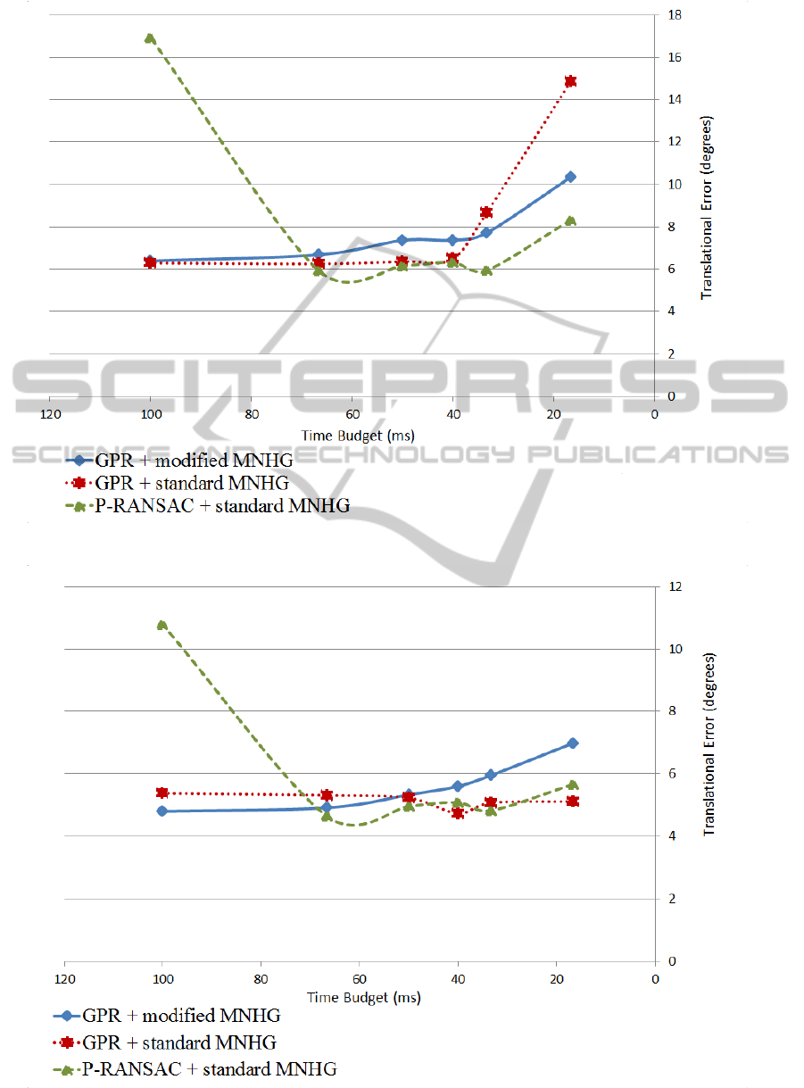
Figure 1: Time budget x Translational error in degrees (forward motion).

Figure 2: Time budget x Translational error in degrees (side-wise motion).

VISAPP2014-InternationalConferenceonComputerVisionTheoryandApplications

412

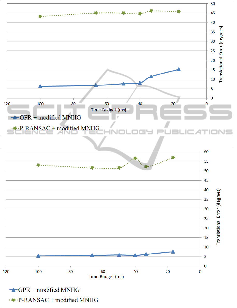
Figure 3: Time budget x Translational error in degrees (forward motion) in a modest device.

Figure 4: Time budget x Translational error in degrees (side-wise motion) in a modest device.

GeneralizedPreemptiveRANSAC-MakingPreemptiveRANSACFeasibleeveninLowResourcesDevices

413

lar hardware conﬁguration. However, once the budget

and the parameters have been deﬁned for a particular

hardware conﬁguration, they can be used for any in-

stance of such system.

6 CONCLUSIONS

In this paper, we proposed the usage of the General-

ized Preemptive RANSAC (GPR), that can be seen

as a generalization of the Preemptive RANSAC (P-

RANSAC), and can be applied successfully to dif-

ferent hardware conﬁgurations, speciﬁcally to low-

budget hardware conﬁgurations.

We concentrated in validate our approach in a con-

trolled scenario in order to assure a high level of conﬁ-

dence in the results since we have the ground truth as a

reference for the comparisons along the several exper-

iments we have performed. The use of two-view ge-

ometry and a single model (cloud of points projected

in two synthetic frames) demonstrated to be adequate

to our needs.

We tested the algorithms on synthetic data, an-

alyzing the average translational error produced for

several time budgets, in order to simulate different

time constraints required by applications with differ-

ent objectives. The ﬂexibility of the GPR allowed

it to maintain lower average error rates even in the

low-budget hardware conﬁguration used. This means

that the ﬂexibility of GPR allows a number of com-

puter/robot vision applications to be developed even

when using modest hardware setups.

Future works include a deeper study of the param-

eter setup to correlate the information and try to esti-

mate a model that can give a range of values for the

model’s parameters in order to decrease the need for

human intervention and decrease the amount of time

needed for the parameter setup. At the end, we ex-

pect to deliver a system able to run a calibration step

in the hardware setup that aids the determination of

adequate parameters for a given time budget in the

selected device. New experiments are been conducted

using real pairs of images to compare the performance

of both approaches under such conditions.

We also plan to investigate the ﬁnding of several

motion models in a single image pair, as well as com-

bining some hypotheses generation methods (e.g. 5-

point, 8-point and homography) in the generation step

in order to promote diversity of hypotheses. This will

make GPR adapted to work with a variable number

of models. We expect that this will provide more re-

liability in the estimation since each model’s motion

may be best estimated by distinct types of hypotheses,

i.e. computed by distinct generation methods, such

as backgrounds mapped by homographies and other

objects mapped by the 8-point algorithm in forward

motion (which surpasses 5-point in such conditions

(

Segvi

c et al., 2007a)).

Finally we plan to perform tests with other hard-

ware platforms, specially those low budget processors

which are been used in autonomous robot vision im-

plementations.

ACKNOWLEDGEMENTS

The authors would like to express gratitude to Profes-

sor Sini

Segvi

c from the University of Zagreb for

all his help and for providing us with his simulation

code, on which we built on. Bruno M. Carvalho is

supported by FAPERN/CNPq PRONEM Grant.

REFERENCES

Chum, O. and Matas, J. (2005). Matching with PROSAC

- Progressive Sample Consensus. In Proceedings of

the 2005 IEEE Computer Society Conference on Com-

puter Vision and Pattern Recognition (CVPR’05) -

Volume 1 - Volume 01, CVPR ’05, pages 220–226,

Washington, DC, USA. IEEE Computer Society.

Chum, O. and Matas, J. (2008). Optimal Randomized

RANSAC. IEEE Transactions on Pattern Analysis

and Machine Intelligence, 30(8):1472–1482.

Fischler, M. A. and Bolles, R. C. (1981). Random Sam-

ple Consensus: A Paradigm For Model Fitting With

Applications to Image Analysis and Automated Car-

tography. Commun. ACM, 24(6):381–395.

Gomes-Neto, S. and Carvalho, B. M. d. (2010). BRUMA:

Generalizing All Preemption Functions. In Proc. IWS-

SIP, pages 380–383.

Konouchine, A., Gaganov, V., and Veznevets, V. (2005).

AMLESAC: A New Maximum Likelihood Robust Es-

timator. In In Proc. Graphicon05, pages 93–100.

Li, H. and Hartley, R. (2006). Five-Point Motion Estima-

tion Made Easy. In Proceedings of the 18th Inter-

national Conference on Pattern Recognition - Volume

01, ICPR ’06, pages 630–633, Washington, DC, USA.

IEEE Computer Society.

Michaelsen, E., von Hansen, W., Meidow, J., Kirchhof, M.,

and Stilla, U. (2006). Estimating The Essential Ma-

trix: GOODSAC versus RANSAC. In Symposium of

ISPRS Commission III: Photogrammetric Computer

Vision, pages 161–166.

Nist

er, D. (2003). Preemptive RANSAC for Live Structure

and Motion Estimation. In Proceedings of the Ninth

IEEE International Conference on Computer Vision -

Volume 2, ICCV ’03, pages 199–, Washington, DC,

USA. IEEE Computer Society.

Nist

er, D. (2004). An Efﬁcient Solution to the Five-Point

Relative Pose Problem. IEEE Trans. Pattern Anal.

Mach. Intell., 26(6):756–777.

VISAPP2014-InternationalConferenceonComputerVisionTheoryandApplications

414

Raguram, R., Frahm, J.-M., and Pollefeys, M. (2008). A

Comparative Analysis of RANSAC Techniques Lead-

ing to Adaptive Real-Time Random Sample Consen-

sus. In Forsyth, D., Torr, P., and Zisserman, A., edi-

tors, Computer Vision ECCV 2008, volume 5303 of

Lecture Notes in Computer Science, pages 500–513.

Springer Berlin Heidelberg.

Rodehorst, V. and Hellwich, O. (2006). Genetic Algo-

rithm SAmple Consensus (gasac) - A Parallel Strat-

egy for Robust Parameter Estimation. In Proceedings

of the 2006 Conference on Computer Vision and Pat-

tern Recognition Workshop, CVPRW ’06, pages 103–,

Washington, DC, USA. IEEE Computer Society.

Torr, P. H. S. and Zisserman, A. (2000). MLESAC: A New

Robust Estimator with Application to Estimating Im-

age Geometry. Computer Vision and Image Under-

standing, 78:2000.

Vedaldi, A., Jin, H., Favaro, P., and Soatto, S. (2005).

KALMANSAC: Robust Filtering by Consensus. In

ICCV, pages 633–640. IEEE Computer Society.

Segvi

c, S., Schweighofer, G., and Pinz, A. (2007a). In-

ﬂuence of numerical conditioning on the accuracy of

relative orientation. In CVPR. IEEE Computer Soci-

ety.

Segvi

c, S., Schweighofer, G., and Pinz, A. (2007b). Per-

formance evaluation of the ﬁve-point relative pose

with emphasis on planar scenes. In Performance

Evaluation for Computer Vision, pages 33–40, Aus-

tria. Workshop of the Austrian Association for Pattern

Recognition.

GeneralizedPreemptiveRANSAC-MakingPreemptiveRANSACFeasibleeveninLowResourcesDevices

415