Image-based Object Classification of Defects in Steel using Data-driven
Machine Learning Optimization
Fabian B¨urger
1
, Christoph Buck
2
, Josef Pauli
1
and Wolfram Luther
2
1
Lehrstuhl Intelligente Systeme, Universit¨at Duisburg-Essen, Bismarckstraße 90, 47057 Duisburg, Germany
2
Lehrstuhl Computergrafik und Wissenschaftliches Rechnen, Universit¨at Duisburg-Essen,
Lotharstr. 63, 47057 Duisburg, Germany
Keywords:
Object Classification, Algorithm Recommendation, Data-driven Hyper-parameter Optimization.
Abstract:
In this paper we study the optimization process of an object classification task for an image-based steel quality
measurement system. The goal is to distinguish hollow from solid defects inside of steel samples by using
texture and shape features of reconstructed 3D objects. In order to optimize the classification results we
propose a holistic machine learning framework that should automatically answer the question “How well
do state-of-the-art machine learning methods work for my classification problem?” The framework consists
of three layers, namely feature subset selection, feature transform and classifier which subsequently reduce
the data dimensionality. A system configuration is defined by feature subset, feature transform function,
classifier concept and corresponding parameters. In order to find the configuration with the highest classifier
accuracies, the user only needs to provide a set of feature vectors and ground truth labels. The framework
performs a totally data-driven optimization using partly heuristic grid search. We incorporate several popular
machine learning concepts, such as Principal Component Analysis (PCA), Support Vector Machines (SVM)
with different kernels, random trees and neural networks. We show that with our framework even non-experts
can automatically generate a ready for use classifier system with a significantly higher accuracy compared to
a manually arranged system.
1 INTRODUCTION
High quality steel is a versatile material that has many
demanding applications such as pipeline tubes, con-
struction and automotive engineering. In order to im-
prove the cleanliness – the quality – of the steel, the
amount of non-metallic inclusions (NMIs) inside of
the product has to be reduced. These inclusions oc-
cur during the production process and usually contain
materials like oxides, sulfides or nitrides.
At first, it is necessary to measure the cleanliness
of steel samples to identify possible sources of con-
tamination in the production line. Currently avail-
able measurement techniques are microscope obser-
vation, sulfur prints, SEM-scans, x-ray and ultrasonic
sound analysis. Usually a high measurement preci-
sion in combination with information about the chem-
ical composition of the NMIs is very time-consuming
and therefore cost-intensive. In (Herwig et al., 2012)
an automated measurement system based on opti-
cal scanning of milled steel surfaces is described.
Thereby a milling machine slices thin layers of 10µm
of a raw steel sample and each layer is imaged with
a resolution of 2.5 – 20µm per pixel. Within these
surface images, sections of different kinds of objects,
namely NMIs, pores, cracks, shrink holes and milling
artifacts can be found. After segmentation of the de-
fects the binary 2D masks on consecutive layers are
connected to obtain a 3D voxel-based reconstruction
of the objects.
The distinction of the different object classes is
crucial since only solid NMIs are relevant for the
cleanliness analysis. Hollow objects like pores –
which occur during treatments of the molten steel
with gases (e.g. argon purging) – and cracks usually
disappear after metal forming of the raw steel prod-
uct. Shape features of the 3D objects in combination
with machine learning can be used to classify objects
into globular objects, cracks and artifacts with an ac-
curacy of 98 – 99% (B¨urger et al., 2013). At first,
it was believed that all detected globular defects are
solid NMIs but microscopy analyses revealed that a
significant number of these objects are hollow (Buck
et al., 2013). The main challenge is that solid NMIs
143
Bürger F., Buck C., Pauli J. and Luther W..
Image-based Object Classification of Defects in Steel using Data-driven Machine Learning Optimization.
DOI: 10.5220/0004737101430152
In Proceedings of the 9th International Conference on Computer Vision Theory and Applications (VISAPP-2014), pages 143-152
ISBN: 978-989-758-004-8
Copyright
c
 2014 SCITEPRESS (Science and Technology Publications, Lda.)

500µm
x
y
z
x
y
z
x
y
z
x
y
z
Figure 1: Texture and 3D voxels of 4 exemplary pores.
x
y
z
x
y
z
x
y
z
x
y
z
Figure 2: Texture and 3D voxels of 4 exemplary solid NMIs.
and hollow pores have a very similar appearance in
the images of the proposed measurement system as
the image resolution is at least a magnitude lower than
the microscopy resolution (≤ 1µm per pixel) used for
manual verification.
The task to design a suitable classification system
is difficult as it is not evenknownif a desired accuracy
performance can be achieved with the given sensor
data. First, it is not clear which texture or shape fea-
tures make a distinction possible. Secondly, a suitable
classifier concept with adequate parameters has to be
chosen to achieve good recognition rates and gen-
eralization abilities. Additionally, dimension reduc-
tion techniques such as Principal Component Analy-
sis may increase the performance of the system. Usu-
ally, a time-consuming development process has to be
done in order to find a good classifier system. This pa-
per targets the problem to automatically obtain such a
classifier system using a holistic machine learning op-
timization framework which realizes a reliable image-
based distinction between NMIs and pores.
2 PROBLEM DESCRIPTION
After the segmentation process a list of n
Obj
objects
is obtained and each object o
i
with 1 ≤i ≤ n
Obj
is de-
scribed with a binary voxel set V
i
(x, y, z) ∈ { 0, 1} and
the 3D gray-value texture array T
i
(x, y, z) ∈ [0, 255].
The object size is D
1
×D
2
×D
3
and 1 ≤ x ≤ D
1
,
1 ≤ y ≤ D
2
and 1 ≤ z ≤D
3
. Example objects of pores
can be found in figure 1 and objects showing NMIs
are depicted in figure 2.
The variation of the object’s appearance in the
class NMIs is especially huge because the compo-
sition of the materials and their size are unknown.
While the differences in the 3D shape are hardly no-
ticeable, the most significant difference is the “tail”
of the solid objects. It can be seen in the texture
below the actual object (see arrows in figure 2). It
originates from the milling cutter crushing the solid
material along the milling grooves. But this tail is
not clearly appearing at every NMI – hence even steel
experts cannot perfectly distinguish pores from solid
NMIs when only seeing their texture and shape at the
system’s relatively low resolution.
2.1 Machine Learning Challenges
The following steps are usually performed in a ma-
chine learning approach to distinguish objects (Jain
et al., 2000). First, a set of objects is labeled from
experts as ground truth. Then a set of meaningful
features is derived that describes especially the dif-
ferences between the classes that should be separated.
Finally, a classifier is trained with the feature vectors
and the ground truth labels.
Our classification task bares typical problems oc-
curring in many machine learning applications. Due
to the high cost for labeling ground truth data (in our
case manual microscopic inspection) only few labels
are available (72 pores and 52 solid inclusions). As it
is not clear which feature set works best on the de-
scribed problems, we use a set of problem-specific
features combined with well-known standard descrip-
tors which are presented in section 4.
The combination of many features is usually high-
dimensional which leads to the curse of dimension-
ality. As only few training samples are available,
high dimensional feature spaces are sampled only
very sparsely and are therefore almost empty (Jain
et al., 2000). Canonical distance measures, like the
Euclidean distance, become less meaningful in high
dimensional spaces (Beyer et al., 1999) which can
lead to a degradation of classifier performance. An-
other effect is the negative influence of irrelevant
and noisy features on the classification performance
which is known as the peaking phenomenon. To over-
come these dimensionality related problems, dimen-
sion reduction techniques have been proposed. The
most common approaches are feature subset selection
or feature transforms, such as Principal Component
Analysis (PCA) (Jain et al., 2000). The feature sub-
set selection approach removes irrelevant dimensions
while a feature transform generates a compressed data
representation based on the geometric properties of
the original data.
The choice of a classifier concept itself determines
the adaptation and generalization abilities (also called
VISAPP2014-InternationalConferenceonComputerVisionTheoryandApplications
144

bias and variance) of the system. Many classifiers ex-
ist, such as naive Bayes classifiers, k-Nearest Neigh-
bor classifiers (kNN), Multilayer Perceptrons (MLP),
Support Vector Machines (SVM) or random trees.
But there is not a single machine learning concept that
performs best on all problems – this is referred to as
the no-free-lunch theorem (Wolpert, 1996). Addition-
ally, most machine learning concepts have various pa-
rameters such as kernel widths or network sizes (see
section 3.3) which havea great influence on the classi-
fier performance. In order to produce optimal results
these parameters have to be tuned for each new clas-
sification problem.
2.2 Related Work
In real world machine learning tasks it is usually
the case that any combination of the aforementioned
problems can occur. It is time-consuming manual
work to evaluate all possible combinations of solu-
tions to achieve the optimal classifier performance.
This is a general hindrance to use classifier systems
in practice as each new data set, a novel feature or a
different sensor may make a revision of the whole sys-
tem necessary. These observations motivate a holis-
tic view on machine learning with an automatic opti-
mization process of the components.
In recent literature there are two categories of ap-
proaches in the context of classifier framework opti-
mization, namely search-based and metalearning al-
gorithms. In search algorithms, a classifier system
is optimized by trying and evaluating a set of the
system’s hyper-parameters. Usually, the final clas-
sifier accuracy based on the training data is used as
the objective function. Different search strategies and
framework components have incorporated within this
optimization process. In (Bergstra and Bengio, 2012)
grid search and random search methods for classi-
fier parameter optimization are compared. Further-
more, an additional feature selection component has
been incorporated using genetic algorithms (Huang
and Wang, 2006), particle swarms (Lin et al., 2008b)
and simulated annealing (Lin et al., 2008a). In (So-
morjai et al., 2004) a larger framework for biomed-
ical spectra classification is proposed that incorpo-
rates data visualization, preprocessing, feature extrac-
tion and selection, classifier development and aggre-
gation. The authors use several strategies to optimize
the hyper-parameters and configurations. However,
their approach is focused especially on the develop-
ment of spectral features and interpretability in the
diagnostics field.
Metalearning is an emerging field in the machine
learning community and deals with the questions
Feature
Selection
Layer
Feature
Transform
Layer
Classifier
Layer
Figure 3: Overview of the layers of the proposed machine
learning framework. The dimensionality is successively re-
duced by the feature selection and feature transform layers
until the classifier returns the final one-dimensional class
label y.
what knowledge can be extracted of specific learn-
ing tasks. An all-encompassing survey of this field
can be found in (Lemke et al., 2013). One core as-
pect of metalearning is algorithm recommendation
based on previous learning tasks. The idea is to es-
tablish a connection between the feature data char-
acteristics and algorithm performance without trying
all possible algorithms. In (Reif et al., 2012) a re-
cent review of automatic classifier selection systems
based on metalearning can be found. They focus on
the simplicity for non-experts to automatically choose
a proper classification pipeline with optimized fea-
ture selection, classifier and parameters. These ap-
proaches use meta-features of the base features to pre-
dict the performance of classifiers on the dataset. Pop-
ular meta-features contain statistical properties of the
base feature vectors such as the number of samples
and classes as well as entropy based distribution met-
rics. Furthermore, so-called landmarking features are
applied as well that use the performance of very sim-
ple classifiers as a descriptor. The approach of met-
alearning is certainly faster than exhaustive search for
the best algorithm, but it relies on the ability of meta-
features to describe the “kind” of data distribution.
Finally, the performance of the meta-classifier may
also suffer from the same aforementioned challenges
which can lead to a bad performance of the suggested
algorithm on the base classification task.
3 DATA-DRIVEN MACHINE
LEARNING FRAMEWORK
3.1 System Concept
In order to overcome all problems mentioned in the
previous sections, we propose a data-drivenand holis-
tic machine learning framework that covers all neces-
sary fields in machine learning, namely feature subset
selection, feature transform, classifier concept, classi-
fier parameters and evaluation with cross-validation.
The coarse system structure is depicted in figure 3.
The main principle of the framework is successive di-
mension reduction which is realized in three layers,
Image-basedObjectClassificationofDefectsinSteelusingData-drivenMachineLearningOptimization
145

Table 1: Framework components on the different layers.
layer components / algorithms
Feature
Selection
dimension reduction using feature
subset F
sub
⊆ F
all
Feature
Transform
{no PCA transform, PCA with n
PCA
dimensions}
Classifier {naive Bayes, random tree, k-nearest
neighbors (kNN), multilayer percep-
tron (MLP), Support Vector Machine
(SVM) with linear and Gaussian ker-
nel}
namely feature selection, feature transform and finally
the classifier layer. Each layer contains one or more
components which are listed in table 1. A system con-
figuration is defined by the selection of one compo-
nent on each layer as well as the components’ specific
parameters. First we describe the forward direction
of the framework when the system configuration is
known and a new instance should be classified. The
optimization of the framework configuration can be
seen as training or learning process and is described
in section 3.4.
3.2 Dimension Reduction
The input for the framework is a feature group which
is a set F
all
= {F
1
, F
2
, . . . , F
N
} containing N features
channels. A feature channel is a vector x
F
i
∈ R
1×n
i
with n
i
≥1 dimensions. This definition allows to han-
dle single feature values as well as higher dimensional
descriptors which occur e.g. in texture features (see
section 4). The concatenated feature vector of a fea-
ture group F
(·)
set is defined as
x
F
(·)
= [x
F
1
, x
F
2
, . . . , x
F
N
] ∈ R
1׈n
, ˆn =
∑
F
i
∈F
(·)
n
i
. (1)
Note that these concatenated feature vectors could di-
rectly be used as an input for classifiers. Feature scal-
ing should be applied to all feature channels as it
improves the classifier performance (Juszczak et al.,
2002). We scale the value domains to a range of [0, 1].
In the first layer the feature subset selection removes
irrelevant features that could disturb the further pro-
cess. The resulting feature subset F
sub
⊆ F
all
is used
to form a concatenated vector x
FS
that is passed to the
feature transform layer.
Feature transforms are a powerful tool to re-
duce the dimensionality with estimating low dimen-
sional manifolds inside of the high dimensional fea-
ture space. The aim is that simple classifiers (e.g. with
linear kernels) may perform better on the transformed
data. An overview of several common linear and non-
linear techniques can be found in (Van der Maaten
et al., 2009). The feature transform layer contains
the Principal Component Analysis (PCA) algorithm.
This is a linear transform that uses a new coordinate
system whose base vectors are ordered by the high-
est statistical variance of the original data. The PCA
can only handle linear correlations of the feature di-
mensions but it has been shown that it works well in
many cases and allows a simple out-of-sample exten-
sion that transforms new feature vectors into the new
coordinate space. If the PCA component is chosen by
the framework training, the new feature vector x
FT
is
formed by using the first n
PCA
dimensions of the PCA
transformed vector of x
FS
. Otherwise, when the PCA
is deactivated, the vector x
FS
is passed directly to the
classifier and x
FT
= x
FS
.
3.3 Classifier Layer
Finally, the classifier layer contains a set of 5 popular
classifier concepts which take the feature vector x
FT
and returns a class label y for the given instance. A
review of recent classifiers in machine learning can be
found in (Jain et al., 2000). Table 1 lists the classifier
concepts that are available in the classifier layer of our
framework.
The naive Bayes classifier is based on the Bayes’
theorem in combination with a Gaussian normal dis-
tribution that assigns the most probable class to an
instance. This classifier has no parameters and works
well for simple classification tasks.
The random tree classifier consists of a tree struc-
ture of decision nodes that check a threshold of single
variables inside of the feature data.
The k-nearest neighbor classifier stores all feature
vectors in the training phase. To classify a new in-
stance it performs a search to find the k closest in-
stances according to a distance metric which can be
e.g. Euclidean or Mahalanobis distance. The parame-
ter k varies the smoothness of the decision boundary.
The multilayer perceptron (MLP) is a feedforward
neural network that consists of several layers which
have itself a number of neurons. The layers are con-
nected with weights that are trained using backprop-
agation so that the network output – the class label
– matches with the input feature vector. The network
size is determined by the number of hidden layers and
the number of neurons per layer.
The Support Vector Machine (SVM) classifier es-
timates a maximum margin decision boundary in the
feature vector space to minimize the risk of misclassi-
fication. It is a powerful concept that can also handle
non-linear classification using kernel functions such
as the Gaussian kernel. We use the ν-SVM (Chang
and Lin, 2011) which has a parameter ν that penal-
izes misclassified instances. Furthermore, we use the
VISAPP2014-InternationalConferenceonComputerVisionTheoryandApplications
146

linear kernel with no additional parameters as well as
the Gaussian kernel with the kernel width γ that con-
trols the smoothness of the decision boundary. Note
that only one classifier is used to classify instances in
a trained framework. Compared to previous frame-
works we investigate the concept of the SVM with
different kernels more deeply.
3.4 Training of the Framework
Configuration
A framework configuration consists of the choice of
active components on each layer (see table 1) as well
as the choice of the corresponding parameters. The
forward direction to classify a new instance is fast
as only one, namely the trained configuration has to
be evaluated. Clearly, it is a challenge to find the
best framework configuration for a given classifica-
tion problem as the number of all possible combina-
tions is exponential and there is no straightforward
way to “guess” the best configuration. Furthermore,
an automatic optimization or training process is de-
sired that does not require expert knowledge. The
goal is that experts may focus on the development of
better features or sensor techniques rather than time-
consuming classifier optimization.
In our framework training process the only thing
the user has to provide is a number of annotated
ground truth instances with their feature sets. As ma-
chine learning in general is an ill-posed problem, one
can describe our training approach as totally data-
driven regularization of all system hyper-parameters.
In order to find a solution in reasonable time, we pro-
pose a partly-heuristic grid search approach with the
classifier performance as objective function. To de-
fine an efficient optimization strategy we use the black
box principle and introduce a machine learning black
box and a classifier black box which are depicted in
figure 4. We separate these to use a different search
strategy for each black box.
3.5 Classifier Black Box
The classifier black box (see figure 4) is the core
component that optimizes the feature transform, the
classifier and its parameters and evaluates the per-
formance of the current system configuration. First,
the classifier black box investigates the effect of the
PCA and performs a grid search with its parameters
n
PCA
= {1, 2, 3, 4, 5, 10}. In order to save computa-
tion time, we choose this list of values as in most fea-
ture sets the intrinsic dimensionality is rather low and
the first few PCA dimensions are usually sufficient.
As an additional configuration, the PCA transform is
Classifier
Feature transform
Features and ground truth labels
Feature subset selection
System performance evaluation
Best system configuration
concept,
parameters
concept,
parameters
concept,
feature sets
Classifier black box
Machine learning black box
Figure 4: Black box structure for the training phase of the
framework. The loop arrows on the right indicate the inves-
tigated method and parameter variations.
skipped and the feature vector x
FS
is directly passed
to the classifier. The classifier is the most important
part of the classifier black box. In every round of
the feature transform grid search we perform a grid
search for each classifier model and its correspond-
ing parameters that are listed in table 2. Grid search
still a popular method in hyper-parameter optimiza-
tion for classifiers with up to two parameters, though
random search methods work better for higher dimen-
sional search spaces (Bergstra and Bengio, 2012).
3.6 System Quality Metric
The system performance evaluation is done for each
feature transform, classifier and parameter combi-
nation using k-fold cross-validation. This method
achieves a good estimation of the classifiers’ bias and
variance at still reasonable computation costs (Jain
et al., 2000). We choose k ≤ 10 such that at least 15
samples remain in the evaluation set. The minimum
size constraint for the evaluation set is necessary for
small sample sizes to avoid undefined values for ac-
curacy, precision and recall. There are several ways to
define a quality metric for the whole classifier system
that serves as objective function for the optimization
process. It is possible to use the overall F-measure
(harmonicmean of precision and recall) or e.g. the ac-
curacy of a specific class. In many frameworks in lit-
erature (see section 2.2) the overall accuracy value is
used. However, we use the average value of accuracy,
precision and recall of all cross-validation rounds to
reward a solution with a high value in all of the three
base metrics. Precision and recall are also very im-
portant quality metrics in many classification tasks.
Image-basedObjectClassificationofDefectsinSteelusingData-drivenMachineLearningOptimization
147

Table 2: Classifier concepts and parameter ranges.
classifier parameter ranges (steps)
Naive Bayes -
Random Tree (Matlab
Statistics Toolbox)
- (self-optimizing with
pruning)
k-nearest neighbors k ∈ [1, 15](15), distance
metric ∈ {Euclidean,
Mahalanobis}
MLP with backpropaga-
tion
number of hidden layers
∈ [0, 2](3), number of neu-
rons per layer ∈[2, 20](6)
ν-SVM with linear
kernel
ν ∈ [0.1, 0.9](9)
ν-SVM with Gaussian
kernel
ν ∈ [0.1, 0.9](9),
γ ∈ [
1
5
,
1
1000
](5)
3.7 Feature Subset Selection
The classifier black box is used to perform feature
subset selection within the machine learning black
box. The classifier black box is already performing
feature transforms to reduce the dimensionality, but
feature selection is an alternative, powerful approach
to optimize the classification performance (Kohavi
and John, 1997). In our experiments in section 5
we show that the performance can be significantly in-
creased using additional feature selection. We choose
wrapper approaches (rather than filters) for feature se-
lection because the final classifier performanceis used
directly. As an exhaustive feature subset selection has
exponential complexity with the number of features,
heuristics help to efficiently decrease the computa-
tional costs. We use simple Sequential Forward and
Backward Selection (SFS and SBS) as well as their
more sophisticated floating extensions to find a good
feature subset F
sub
. SFS starts with an empty subset
and consecutively adds the features which achieves
the best quality metric when combined with the cur-
rent subset. SBS starts with the full set and sequen-
tially removes features. Sequential Floating Forward
and Backward Selection (SFFS and SFBS) use these
two simple strategies to obtain backtracking capabili-
ties and achieve near-optimal solutions at reasonably
higher costs (Jain et al., 2000). As each feature chan-
nel of the feature group F
all
= {F
1
, F
2
, . . . , F
N
} is not
limited to one dimension (see section 4), the feature
subset selection only selects whole channels to save
computational time.
3.8 Training Complexity
We start with the complexity of the classifier black
box optimization. Let C
i
be the ith classifier of the
classifier set C. The complexities of the classifier
training and evaluation are denoted as f
Train
(·) and
f
Eval
(·), respectively. Of course, they also depend on
the training set and the current feature subset
˜
F
s
. Us-
ing k-fold cross-validation, the complexity for a sin-
gle classifier evaluation and one combination of pa-
rameters
˜
P becomes
f
Param
(C
i
,
˜
F
s
,
˜
P) = k ·( f
Train
(C
i,
˜
F
s
,
˜
P
) + f
Eval
(C
i,
˜
F
s
,
˜
P
)).
(2)
The classifier C
i
has the set of P
i
parameters and each
parameter has a sampling set P
i, j
of values. Testing
all parameter combinations, the Cartesian product has
to be considered and the complexity for all classifiers
and all of their parameters is
f
Classifiers
(
˜
F
s
) =
|C|
∑
i=1
""
|P
i
|
∏
j=1
|P
i, j
|
#
· f
Param
(C
i
,
˜
F
s
,
˜
P)
#
.
(3)
Additionally, the tier of feature transforms with n
FT
combinations leads to a total complexity of the clas-
sifier black box of
f
ClassifierBlackbox
(
˜
F
s
) = n
FT
· f
Classifiers
(
˜
F
s
). (4)
Using the classifiers and parameters of table 2 as well
as the preprocessing steps, a total amount of 728 com-
binations is tested. As these steps are independent of
each other, they can easily be parallelized.
Finally, the feature subset selection step of n
F
fea-
tures is performed. Testing all combinations would
lead to a total complexity of O(2
n
F
) and is only feasi-
ble for small feature sets. The simple selection strate-
gies SFS and SBS have a determined number of it-
erations of
1
2
(n
2
F
+ n
F
). Using floating methods the
number of iterations depends on the actual quality re-
sults but is higher (though still polynomial) due to the
combination of SFS and SBS.
4 OBJECT FEATURES
In order to distinguish pores from NMI objects, we
derive 17 texture and shape features while the idea
is to combine problem-specific features with stan-
dard state-of-the-art descriptors. The feature subset
selection chooses the most promising feature subset.
Therefore, the classification results most likely bene-
fit from a large feature pool, though the computation
time for the feature selection increases.
4.1 Texture Features
The tail of solid objects (described section 2) is a
promising feature that we describe in the following
way. First, the main direction of the milling pattern is
estimated using the 2D Fourier transform. The spec-
trum shows a wedge shaped area of high magnitudes
VISAPP2014-InternationalConferenceonComputerVisionTheoryandApplications
148

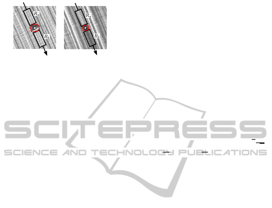
(a) Pore. (b) NMI with tail.
Figure 5: Areas for texture analysis of the tail indicator. The
arrows indicate the main pattern direction. For many NMIs
(b) the texture in R
b
is darker than in R
a
.
which can be used to robustly estimate the main angle
of the pattern even in presence of noise (Herwig et al.,
2012). As depicted in figure 5, two rectangular areas
are defined containing the texture before (R
a
) and af-
ter (R
b
) the object in direction of the milling pattern.
The tail indicator is calculated by dividing the aver-
age gray value inside of area R
b
by the one of area
R
a
. This value is very close to 1 for pores and signif-
icantly lower (between 0.5 and 0.8) for NMIs with a
visible tail.
Additionally, we use standard texture features,
namely the mean and standard deviation of the gray
values inside of the object. Local binary patterns
(LBP) are a popular state-of-the-art description of tex-
tures. Generally, LBP descriptors analyze the bright-
ness differences of a pixel and its direct neighbor-
hood. The pattern is encoded to a binary string and
aggregated to a descriptor histogram counting the
frequencies of the pattern configurations. Several
variants have been introduced (Doshi and Schaefer,
2012). We use the rotation invariant, uniform LBP
with 8 neighbors and a radius of 1 which yields a rel-
atively low descriptor dimension of 10 bins. We com-
pute a histogram for each layer of the object and use
the average histogram as a feature.
4.2 Shape Features
As NMI objects have different material properties
than pores, their shape appears less round but more
“jagged” (see figure 1 and 2). To find a proper de-
scription we use several features derived from the bi-
nary voxel array V(x, y, z). The Minkowski function-
als are a set of motion-invariant additive and contin-
uous functionals which form a complete system on
the set of objects that are unions of a finite number
of convex bodies. A single voxel can be considered
as convex body, therefore this definition can be ap-
plied to a connected voxel set like our 3D objects be-
cause it is a union of convex bodies. For the three-
dimensional case the Minkowski functionals are the
volume V, the surface area S, the mean curvature M
(which is proportional to the mean breadth for convex
particles) and the Euler number χ. Roughly speaking,
the Euler number is the number of connected compo-
nents minus the number of tunnels, plus the number
of cavities. For the calculation of these features the
reader is referred to (Buck et al., 2013). We define
the density of the Minkowski functionals as a frac-
tion of the particular functional over the total number
of voxels of the minimal bounding box of the defect.
Doing so we achieve a normalization of the function-
als. Furthermore the densities can give interesting in-
sights of the structure of the defects. For example
the density of the surface area for a defect occupy-
ing the same volume as another defect will increase,
when the surface is rougher, i.e. consists of more
voxel configurations with diagonal neighbors, and ap-
proaches infinity for a fractal structure. This might be
a useful feature for automatic classification. Based
on the Minkowski functionals we can calculate the
isoperimetric shape factors given by f
1
= 6
√
π
V
√
S
3
,
f
2
= 48π
2
V
M
3
and f
3
= 4π
S
M
2
which are measures for
the sphericity of 3D objects. The values of f
1
, f
2
and
f
3
are close to 1 for spheres.
Furthermore, we derive the box dimension of the
voxel set for each object. The box dimension is an
empirical estimation of the upper bound of the Haus-
dorff dimension (Falconer, 2003). The Hausdorff di-
mension can be used to describe the intrinsic dimen-
sion or “porosity” of fractal objects.
We also use a voxel configuration histogram of
the object border shape. In a 2×2×2 neighborhood
there are 256 different binary voxel configurations.
The configuration can be described in a similar way
to LBP using the binary string (Ohser and M¨ucklich,
2000)
g(x, y, z) = 2
0
·V(x, y, z) + 2
1
·V(x+ 1, y, z)+
2
2
·V(x, y+ 1, z)+ 2
3
·V(x+ 1, y+ 1, z)+
2
4
·V(x, y, z+ 1) + 2
5
·V(x+ 1, y, z+ 1)+
2
6
·V(x, y + 1, z+ 1) + 2
7
·V(x+ 1, y+ 1, z+ 1).
(5)
Obviously, there are 256 different values whose fre-
quencies are – similar to LBP – stored into a his-
togram. This histogram can be compressed by com-
bining symmetric cases to obtain a 22 dimensional,
rotation-invariant histogram (Toriwaki and Yoshida,
2009). Another way of describing the coarseness of
objects is to compute a variant of the morphological
gradient. We use a 3D opening operation with a ball-
shaped structuring element of radius 2 and count the
additional voxels compared to the initial binary vol-
ume. To obtain a size-invariant metric, we normalize
this number by the total number of voxels.
Image-basedObjectClassificationofDefectsinSteelusingData-drivenMachineLearningOptimization
149

Table 3: Best classification results of the classifier black box without automatic feature selection.
Feature set classifier, parameters, PCA accuracy / precision
/ recall
only tail indicator SVM Gauss, ν=0.5, γ=0.001,
no PCA transform
0.912 / 0.899 / 0.911
all texture features: gray-value mean, gray-value std, tail
indicator, LBP histogram
SVM linear, ν=0.2, PCA,
n
PCA
= 10
0.920 / 0.936 / 0.895
all shape features: volume, morphological gradient, surface
area, surface density, mean breadth, Euler number (6 neigh-
borhood), Euler number (26 neighborhood), sphericity f
1
,
sphericity f
2
, sphericity f
3
, voxel configuration 256, voxel
configuration 22, box dimension
random tree, no PCA transform 0.654 / 0.653 / 0.641
all 17 features random tree, no PCA transform 0.831 / 0.823 / 0.822
5 EXPERIMENTS AND RESULTS
5.1 Classifier Black Box Evaluation
First, we evaluate the classifier black box alone with-
out the feature selection layer (see figure 4). We per-
form a “manual” feature subset selection and com-
pare the classifier optimization results in table 3. The
promising tail indicator alone already reaches an ac-
curacy of 0.912 which shows that the tail is a key de-
scriptor for the NMIs. The accuracy increases only
slightly when the other texture features are used, too.
The shape features alone perform poorly when they
are concatenated. Finally, when using the simple
combination of all 17 presented features, the accu-
racy drops significantly compared to the case when
only the texture features are used. The influence of
the PCA is also marginal in this scenario as it is only
chosen once for the texture features. These effects
indicate that some shape features contain irrelevant
information that disturb the dimension reduction and
classifier algorithms.
The SVM concept performs best on the texture
features, but when shape features are used, the ran-
dom tree classifier achieves the best results. This
shows that the texture features can be separated
“smoothly” and the complete set of shape features
needs a rather complex decision boundary as espe-
cially the voxel configuration histograms are high-
dimensional. When all 17 features are used the total
feature vector space has 302 dimensions.
5.2 Feature Subset Selection
In the next experiment, all features are inside of the
selection pool for the feature subset selection of the
machine learning black box (see figure 4). We com-
pare SFS, SBS and the floating versions SFFS and
SFBS. The best classification results can be found
in table 4. The performance increases in every case
when feature selection is used. However, the results
of the different selection strategies show noticeable
differences. The highest performance is achieved by
the SFFS selection strategy with an accuracy of 0.967.
In most metrics, the forward selection strategies per-
form better than the backward selection algorithms.
The selected subsets show a different number of items
(5 – 10 features) as well as a different selection. This
indicates that the subset selection strategies may get
stuck in local minima, though the differences in ac-
curacy are not extreme. The classifier concepts show
that the SVM is dominating the best solutions, though
its kernel parameters vary. But the MLP and the
kNN classifiers appear in the top 10 result rankings,
too. Here the feature transform layer has more influ-
ence and the PCA is chosen in many configurations
which supports the order of our framework structure
in which the feature selection is applied before the
feature transform.
We can use the selected feature subsets with the
top ranks (table 4 only shows rank 1) to obtain a fea-
ture relevance ranking. In table 5 the occurrences of
each feature in the best 20 subsets of all selection
strategies are counted. This ranking strategy is es-
pecially interesting because the feature combinations
and the final classifier quality are considered. In our
example, the tail indicator has been selected every
time and the Minkowski functionals have also been
chosen very frequently. The high dimensional his-
tograms of the texture and the voxel configurationsal-
most never appear in the best solutions so their usage
degrades the classifier performance and should not be
used.
As the theoretical complexity of the approach is
relatively high, we evaluated the processing times and
feature selection steps. Using an Intel Xeon CPU with
6 × 2.50GHz and Matlab, the average computation
time for a single classifier black box optimization is
74.3 ± 38.4 seconds. The feature selection uses this
VISAPP2014-InternationalConferenceonComputerVisionTheoryandApplications
150

Table 4: Best classification results of the machine learning black box with different feature selection strategies.
selection
strategy
selected feature subset classifier, parameters, PCA accuracy / precision
/ recall
SFS box dimension, Euler number (6 neighbor-
hood), sphericity f
1
, sphericity f
3
, surface
density, tail indicator
SVM linear, ν=0.2, PCA,
n
PCA
= 3
0.944 / 0.953 / 0.944
SBS box dimension, Euler number (6 neighbor-
hood), Euler number (26 neighborhood),
gray-value std, mean breadth, morphologi-
cal gradient, sphericity f
3
, surface density, tail
indicator, volume
SVM Gauss, ν=0.3, γ=0.1,
PCA, n
PCA
= 5
0.943 / 0.945 / 0.946
SFFS box dimension, Euler number (6 neighbor-
hood), mean breadth, sphericity f
2
, sphericity
f
3
, surface area, surface density, tail indicator,
volume
SVM Gauss, ν=0.4, γ=0.001,
no PCA transform
0.967 / 0.970 / 0.962
SFBS mean breadth, sphericity f
2
, surface density,
tail indicator, volume
SVM Gauss, ν=0.3, γ=0.002,
PCA, n
PCA
= 2
0.952 / 0.954 / 0.953
0 100 200 300 400
0.65
0.7
0.75
0.8
0.85
0.9
0.95
1
subset selection iteration
best quality metric
SFS ( best solution in 1.07 hours)
SBS ( best solution in 2.96 hours)
SFFS ( best solution in 3.73 hours)
SFBS ( best solution in 7.30 hours)
Figure 6: Progress and processing time of the classification
quality depending on the subset selection strategy.
optimization and so the number of iterations needed
is important. Figure 6 shows the progress of the best
quality metric (see section 3.5) during the feature se-
lection. The forward strategies (SFS and SFFS) need
far less iterations to select a good subset which shows
that only relatively few features are needed to solve
the example classification task. Reasonably good sub-
sets can be selected using SFS within around one hour
of computation time while the fine-tuning of the SFFS
needs almost 4 hours to find the overall best combina-
tion.
6 CONCLUSIONS
We presented a holistic machine learning framework
that incorporates key machine learning components,
namely classifier and parameters, feature transform
and feature subset selection. The framework auto-
matically optimizes the best configuration using a to-
tally data-driven search strategy. The user just needs
to provide a set of labeled ground truth feature vec-
Table 5: Feature relevance ranking by counting the percent-
aged occurrence in the top 20 results of the feature selection
strategies (SFS, SBS, SFFS, SFBS).
rank feature %
1 tail indicator 100.00
2 surface density 97.50
3 Euler number (6 neighborhood) 80.00
4 mean breadth 71.25
5 box dimension 62.50
6 sphericity f
3
57.50
7 volume 55.00
8 sphericity f
1
52.50
9 Euler number (26 neighborhood) 47.50
10 surface area 46.25
11 gray-value std 42.50
12 sphericity f
2
33.75
13 morphological gradient 28.75
14 gray-value mean 11.25
15 LBP histogram 1.25
16 voxel configuration 256 0.00
17 voxel configuration 22 0.00
tors. We could successfully show the benefits of the
proposed approach with an image-based object clas-
sification task. By passing feature vectors and ground
truth labels, the optimization framework returns the
best classifier pipeline that can be directly used. As
a “byproduct” the proposed feature relevance ranking
provides insight into the most distinctive descriptors
of the classification problem. This knowledge can be
used to develop better features. The framework can
also be used as a feasibility study for classification
problems to check if the measured data and the fea-
tures are able to achieve a required classification ac-
curacy. Using this framework, the machine learning
component becomes a black box so that experts can
focus on the development of task-specific features.
The framework uses party heuristic grid search, so
the complexity of the proposed approach is relatively
Image-basedObjectClassificationofDefectsinSteelusingData-drivenMachineLearningOptimization
151

high. On the other hand, our experiments showed that
it is computationally feasible on today’s computer ar-
chitectures for up to 20 features. The framework is
in every case faster than a manual optimization by an
expert. A fully exhaustive search of all feature se-
lection combinations is clearly infeasible. Due to the
huge parameter search space of the framework, e.g.
evolutionary or random optimization strategies have
a great potential in this approach. In future work,
the framework will be applied to a larger variety of
classification tasks to show its universality. Further-
more, the best classifiers can be combined to obtain
an ensemble classifier (Jain et al., 2000) with a poten-
tially greater predictive performance. Additionally,
the framework can easily be extended with the newest
state-of-the-art classifiers, feature transform and se-
lection algorithms as “plugins”.
REFERENCES
Bergstra, J. and Bengio, Y. (2012). Random search for
hyper-parameter optimization. J. Mach. Learn. Res.,
13(1):281–305.
Beyer, K., Goldstein, J., Ramakrishnan, R., and Shaft, U.
(1999). When is ”nearest neighbor” meaningful? In
Beeri, C. and Buneman, P., editors, Database Theory
ICDT99, volume 1540 of Lecture Notes in Computer
Science, pages 217–235. Springer Berlin Heidelberg.
Buck, C., B¨urger, F., Herwig, J., and Thurau, M. (2013).
Rapid inclusion and defect detection system for large
steel volumes. ISIJ International, 53, No. 11. ac-
cepted.
B¨urger, F., Herwig, J., Thurau, M., Buck, C., Luther, W.,
and Pauli, J. (2013). An auto-adaptive measurement
system for statistical modeling of non-metallic inclu-
sions through image-based analysis of milled steel
surfaces. In Bosse, H. and Schmitt, R., editors,
ISMTII 2013, 11th International Symposium on Mea-
surement Technology and Intelligent Instruments. Ap-
primus Wissenschaftsverlag.
Chang, C.-C. and Lin, C.-J. (2011). LIBSVM: A library
for support vector machines. ACM Transactions on
Intelligent Systems and Technology, 2:27:1–27:27.
Doshi, N. and Schaefer, G. (2012). A comparative analysis
of local binary pattern texture classification. In Visual
Communications and Image Processing (VCIP), 2012
IEEE, pages 1–6.
Falconer, K. (2003). Fractal geometry: mathematical foun-
dations and applications. Wiley, 2 edition.
Herwig, J., Buck, C., Thurau, M., Pauli, J., and Luther,
W. (2012). Real-time characterization of non-metallic
inclusions by optical scanning and milling of steel
samples. In Proc. of SPIE Vol, volume 8430, pages
843010–1.
Huang, C.-L. and Wang, C.-J. (2006). A GA-based fea-
ture selection and parameters optimizationfor support
vector machines. Expert Systems with Applications,
31(2):231 – 240.
Jain, A., Duin, R. P. W., and Mao, J. (2000). Statistical
pattern recognition: a review. Pattern Analysis and
Machine Intelligence, IEEE Transactions on, 22(1):4–
37.
Juszczak, P., Tax, D., and Duin, R. (2002). Feature scal-
ing in support vector data description. In Proc. ASCI,
pages 95–102. Citeseer.
Kohavi, R. and John, G. H. (1997). Wrappers for feature
subset selection. Artificial Intelligence, 97(12):273 –
324.
Lemke, C., Budka, M., and Gabrys, B. (2013). Metalearn-
ing: a survey of trends and technologies. Artificial
Intelligence Review, pages 1–14.
Lin, S.-W., Lee, Z.-J., Chen, S.-C., and Tseng, T.-Y.
(2008a). Parameter determination of support vector
machine and feature selection using simulated anneal-
ing approach. Applied Soft Computing, 8(4):1505 –
1512. Soft Computing for Dynamic Data Mining.
Lin, S.-W., Ying, K.-C., Chen, S.-C., and Lee, Z.-J. (2008b).
Particle swarm optimization for parameter determina-
tion and feature selection of support vector machines.
Expert Systems with Applications, 35(4):1817 – 1824.
Ohser, J. and M¨ucklich, F. (2000). Statistical analysis of
microstructures in materials science. John Wiley New
York.
Reif, M., Shafait, F., Goldstein, M., Breuel, T., and Den-
gel, A. (2012). Automatic classifier selection for non-
experts. Pattern Analysis and Applications, pages 1–
14.
Somorjai, R. L., Alexander, M. E., Baumgartner, R., Booth,
S., Bowman, C., Demko, A., Dolenko, B., Man-
delzweig, M., Nikulin, A. E., Pizzi, N., Pranckevi-
ciene, E., Summers, A. R., and Zhilkin, P. (2004).
A data-driven, flexible machine learning strategy for
the classification of biomedical data. In Dubitzky, W.
and Azuaje, F., editors, Artificial Intelligence Methods
And Tools For Systems Biology, volume 5 of Compu-
tational Biology, pages 67–85. Springer Netherlands.
Toriwaki, J. and Yoshida, H. (2009). Fundamentals of three-
dimensional digital image processing. Springer.
Van der Maaten, L., Postma, E., and Van Den Herik, H.
(2009). Dimensionality reduction: A comparative re-
view. Journal of Machine Learning Research, 10:1–
41.
Wolpert, D. H. (1996). The lack of a priori distinctions
between learning algorithms. Neural computation,
8(7):1341–1390.
VISAPP2014-InternationalConferenceonComputerVisionTheoryandApplications
152