
Event-driven Dynamic Platform Selection for
Power-aware Real-time Anomaly Detection in Video
Calum G. Blair
1
and Neil M. Robertson
2
1
Institute for Digital Communications, University of Edinburgh, Edinburgh, U.K.
2
Visionlab, Heriot-Watt University, Edinburgh, U.K.
Keywords:
FPGA, GPU, Anomaly Detection, Object Detection, Algorithm Mapping.
Abstract:
In surveillance and scene awareness applications using power-constrained or battery-powered equipment, per-
formance characteristics of processing hardware must be considered. We describe a novel framework for
moving processing platform selection from a single design-time choice to a continuous run-time one, greatly
increasing flexibility and responsiveness. Using Histogram of Oriented Gradients (HOG) object detectors and
Mixture of Gaussians (MoG) motion detectors running on 3 platforms (FPGA, GPU, CPU), we characterise
processing time, power consumption and accuracy of each task. Using a dynamic anomaly measure based on
contextual object behaviour, we reallocate these tasks between processors to provide faster, more accurate de-
tections when an increased anomaly level is seen, and reduced power consumption in routine or static scenes.
We compare power- and speed- optimised processing arrangements with automatic event-driven platform se-
lection, showing the power and accuracy tradeoffs between each. Real-time performance is evaluated on a
parked vehicle detection scenario using the i-LIDS dataset. Automatic selection is 10% more accurate than
power-optimised selection, at the cost of 12W higher average power consumption in a desktop system.
1 INTRODUCTION
Opportunities for the use of advanced computer vi-
sion algorithms have increased to include surveillance
and monitoring applications. We consider the de-
ployment of such algorithms in a scenario with lim-
ited electrical power available for processing, such as
surveillance from a mobile vehicle which may be run-
ning on battery power. Timely and accurate detections
of objects and events are still important in such cir-
cumstances. Field Programmable Gate Arrays (FP-
GAs) and Graphics Processing Units (GPUs) offer
large improvements in speed and power compared to
a reference implementation on a standard CPU. This
is increasingly relevant given the growing trend for
smart cameras with processing capability, and the de-
velopment of mobile general-purpose GPUs. Each al-
gorithm implementation on one of these architectures
will have its own performance characteristics — pro-
cessing time, power consumption and algorithm ac-
curacy — and will exist at a certain point in a multi-
dimensional design space.
Using a heterogeneous system which contains
both FPGAs and GPUs offers increased flexibility, al-
lows decisions about the optimal platform to use to
be moved from design time to run-time, and allows
this decision to be updated in response to changing
characteristics within the image or environment. In
this paper, we use detection of parked vehicles in
surveillance video as an anomaly detection applica-
tion. First, we define an anomaly measure based on
the motion of objects within a video. Using a hetero-
geneous system to process video, we select process-
ing platforms — and hence alter system power, speed
and accuracy characteristics — based on this anomaly
level. We show how platform selection changes in
response to changing anomaly levels, and compare
the performance of this dynamically-mapped system
against a static one optimised for power or speed. To
summarise, the contributions of this work are: we de-
scribe our system consisting of multiple implementa-
tions of various object detection algorithms running
across various accelerators in a heterogeneous hard-
ware platform, demonstrate dynamic selection be-
tween these implementations in response to events
within a scene, and describe the associated tradeoffs
between power consumption and accuracy in a real-
time system. This paper is laid out as follows: after
describing relevant work in this section, 2 describes
each algorithm used in the system and their perfor-
54
Blair C. and Robertson N..
Event-driven Dynamic Platform Selection for Power-aware Real-time Anomaly Detection in Video.
DOI: 10.5220/0004737400540063
In Proceedings of the 9th International Conference on Computer Vision Theory and Applications (VISAPP-2014), pages 54-63
ISBN: 978-989-758-009-3
Copyright
c
2014 SCITEPRESS (Science and Technology Publications, Lda.)

mance characteristics. Once an overall anomaly level
is obtained, the mapping procedure described in 3
selects the next set of implementations. We discuss
methodology in 4, results are presented in 5 and fol-
lowed by analysis of the findings in 6. We conclude
with pointers to future work in 7.
We consider first the architectural background of
this work, and then place it in the context of other
parked vehicle detection work evaluated on the same
dataset. FPGAs and GPUs are two of the most com-
mon ways of improving performance of compute-
intensive signal processing algorithms. In general,
FPGAs offer a large speedup over reference imple-
mentations and draw low power because they in-
stantiate logic which closely matches the applica-
tion. However, their use of arbitrary-precision fixed-
point arithmetic can impact accuracy slightly, and
they require specialised knowledge to program, of-
ten incurring longer development times (Bacon et al.,
2013). In contrast, GPUs have a software program-
ming model, using large arrays of floating-point units
to process data quickly, at the expense of power con-
sumption. Their ubiquitous presence in PCs and lap-
tops has made uptake very common in recent years,
and the availability of Nvidia’s CUDA language for
both desktop and (in the near future) mobile and tablet
devices greatly increases the potential for pervasive
vision computing.
When building a system to perform a process-
ing task, we consider each of the characteristics of
FPGA and GPU and select the system which best suits
our application, for example prioritising fast runtime
over low power consumption. This has been done for
various smaller algorithms, such as colour correction
and 2-D convolution, as in (Cope et al., 2010). This
design-time selection can also be done at a low level
using an optimisation algorithm as shown by (Bouga-
nis et al., 2009), although this is usually more con-
cerned with FPGA area vs. latency tradeoffs. As an
example, 1 shows design space exploration for power
and time characteristics of implementation combina-
tions used in this paper, with a well-defined Pareto
curve at the left-hand side. To the authors’ knowl-
edge, little work has been done in the area of power-
aware algorithm scheduling at runtime; the most ap-
propriate is arguably (Yu and Prasanna, 2002), al-
though this does not consider more than two perfor-
mance characteristics or deal with changing optimisa-
tion priorities over time.
The UK Home Office supplies the i-LIDS
dataset (Home Office Centre for Applied Science and
Technology, 2011) used in 5, and this has been used
for anomaly detection by other researchers. (Albiol
et al., 2011) identify parked vehicles in this dataset’s
0
50
100
150
200
250
300
350
400
450 500 550 600 650
180
190
200
210
220
230
processing time (ms)
system power consumption (W)
ped-ggg ped-cff ped-gff ped-gfg ped-cfc
ped-ccc
car-ggg
car-cfc car-gfg
car-ccc
Figure 1: Design space exploration for power vs. time trade-
offs for all possible combinations of car, pedestrian and mo-
tion detector implementations. Pedestrian implementations
are labelled by colour, and car implementations by shape.
PV3 scenario with precision and recall of 0.98 and
0.96 respectively. However, their approach is consid-
erably different from ours, in that they:- (a) require
all restricted-parking lanes in the image to be manu-
ally labelled first, (b) only evaluate whether an object
in a lane is part of the background or not, and (c) do
not work in real-time or provide performance infor-
mation. In addition, their P and R results do not de-
note events, but rather the total fraction of time during
which the lane is obstructed. Due mainly to limita-
tions within our detectors, our accuracy results alone
do not improve upon this state-of-the-art, but given
the points noted above, we are arguably trying to ap-
proach a different problem (anomaly detection under
power and time constraints) than Albiol et al..
2 SYSTEM COMPONENTS
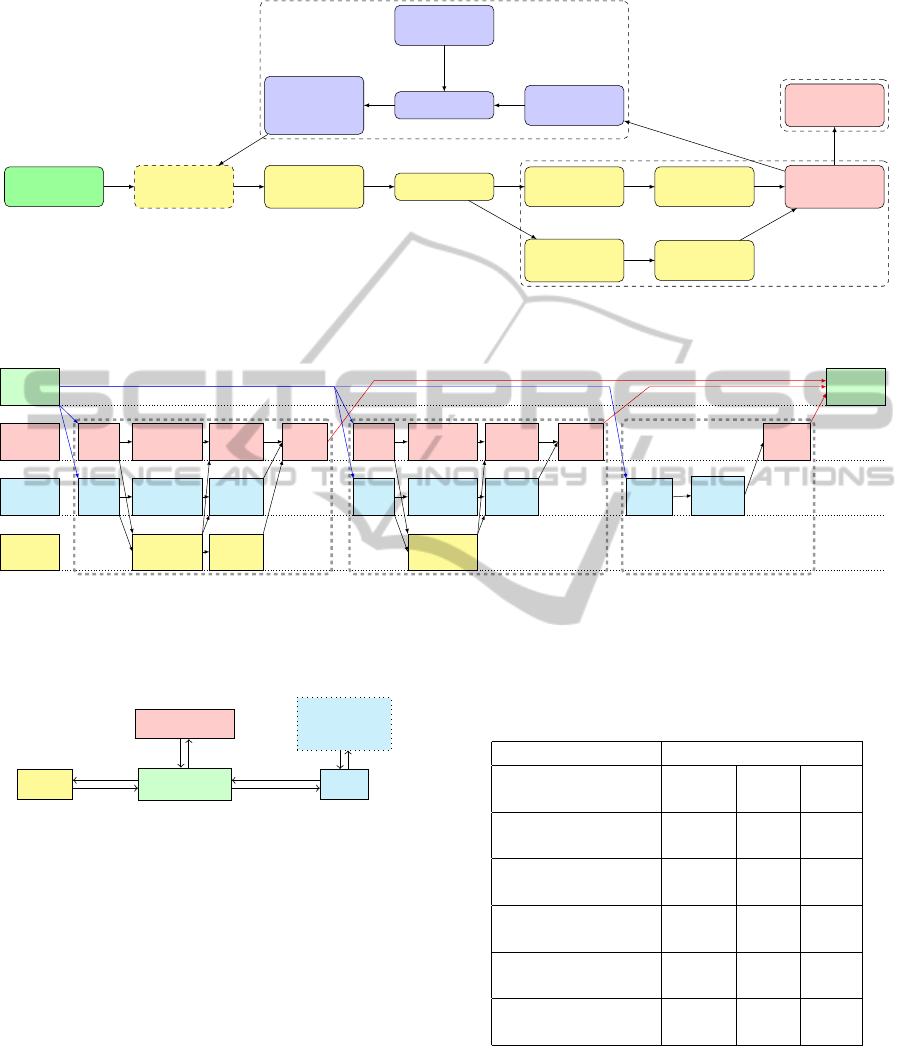
A flow diagram for the high-level frame processing
framework is shown in 2. It works on offline videos
and dynamically calculates the number of frames to
drop to obtain real-time performance at 25FPS. (We
do not count video decode time or time for output im-
age markup and display as part of processing time.)
The ‘detection algorithms’ block generates bounding
boxes with type information, which is used by the re-
maining algorithm stages. (An expanded version of
this step showing all combinations is shown further on
in 4.) This section gives details of each algorithm in
1, i.e. the detection algorithms run on the image, and
method for calculating image anomaly level. The ob-
ject detectors and background subtractor were by far
the most computationally expensive algorithm stages,
so each of these had at least one accelerated version
available. We use a platform containing a 2.4GHz
dual-core Xeon CPU, a nVidia GeForce 560Ti GPU,
and a Xilinx ML605 board with a XC6VLX240T
FPGA, as shown in 3. Implementation performance
Event-drivenDynamicPlatformSelectionforPower-awareReal-timeAnomalyDetectioninVideo
55
performance
data
algorithm
→ platform
mapping
impl. search
priority
selection
log event and
save image
video
frame
detection
algorithms
detection
merging
object tracking
trajectory
clusters
cluster
anomalousness
anomaly
thresholding
location
context update
object
anomalousness
Mapping generation
Anomaly detection
System output
Figure 2: Frame processing and algorithm mapping loop in anomaly detection system.
image
detections
cpu
operation:
scale
histograms classify
group
scale
histograms classify
group
extract
BBs
gpu op-
eration:
scale
histograms classify
scale
histograms classify
update
mask
image
opening
fpga op-
eration:
histograms classify histograms
Pedestrian Detection (HOG) Car Detection (HOG) Motion Detection (MOG2)
Figure 4: All possible mappings of image processing algorithms to hardware. Multiple possible implementation steps within
one algorithm are referred to by the platform they run on. Running HOG with a resize step on GPU, histograms on FPGA
and classification on GPU is referred to throughout as gfg. Data transfer steps not shown.
host x86 CPU
GPU on-card
memory
FPGA
host memory
GPU
PCIe PCIe
Figure 3: Arrangement of accelerated processors within
heterogeneous system. Each processor can access host main
memory over PCI express, and the two accelerators have
private access to on-card memory.
characteristics are shown in 2 where appropriate.
2.1 Pedestrian Detection with HOG
We use various accelerated versions of the His-
tograms of Oriented Gradients pedestrian detector de-
scribed in (Dalal and Triggs, 2005); this algorithm is
well-understood and has been characterised on vari-
ous platforms. Each version is split into three compu-
tationally expensive parts (image resizing, histogram
generation and support vector machine (SVM) clas-
sification), and these are implemented across differ-
ent processing platforms (FPGA, GPU and CPU) as
Table 1: Algorithms and implementations used in the sys-
tem.
Algorithm Implementation(s)
Ped. Detection: FPGA GPU CPU
HOG (§2.1)
Car Detection: FPGA GPU CPU
HOG (§2.2)
Motion Segment: GPU
MoG (§2.3)
Tracking: Kalman CPU
Filter (§2.5)
Trajectory CPU
Clustering (§2.6)
Bayesian Motion CPU
Context (§2.7)
described by (Blair et al., 2013). These mappings
are shown in the left hand side of 4. The following
mnemonics are used in this Figure and elsewhere: a
single implementation is referred to by the architec-
ture each part runs on, e.g. running HOG with resizing
on CPU, histogram generation on FPGA and classifi-
cation on CPU is cfc. Each implementation has dif-
VISAPP2014-InternationalConferenceonComputerVisionTheoryandApplications
56
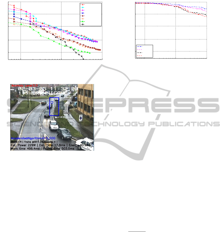
10
−2
10
−1
10
0
0.40
0.50
0.64
0.80
1
false positives per image (FPPI)
miss rate
62% cff
61% gff
59% gfg
59% cfc
53% ccc
52% ggg
48% ggg−kernel
46% Orig−HOG
Figure 5: DET curve (False positives per image against miss
rate) for HOG pedestrian detector.
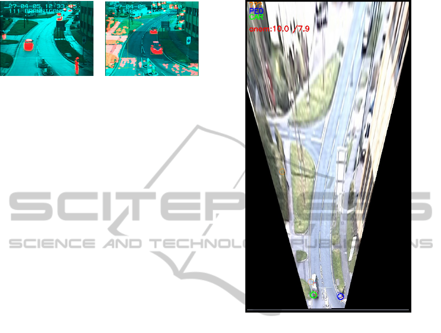
Figure 6: False positives (blue rectangle representing pedes-
trian) from object detectors affected training and testing per-
formance, both directly and through learned context mea-
sures.
ferent power consumption, speed and accuracy char-
acteristics, summarised in 2. These could be switched
between dynamically at runtime with no performance
penalty. We show a False Positives Per Image (FPPI)
curve for each implementation in 5. Detector errors
(e.g. in 6) affect overall accuracy dramatically. Errors
in the training phase also affect the clusters and con-
text heatmaps in 2.6 and 2.7.
2.2 Car Detection with HOG
The HOG algorithm was again selected for car de-
tection due to the presence of existing implemen-
tations running in near-realtime across multiple ar-
chitectures. The CPU and GPU implementations of
HOG on OpenCV were modified to use the parame-
ters in (Dalal, 2006) for car detection. A FPGA ver-
sion was also implemented by modifying the cfc and
gfg versions in (Blair et al., 2013).
These implementations were trained on data from
the 2012 Pascal Visual Object Classes Challenge (Ev-
eringham et al., 2009). The SVM was learned as de-
scribed in (Dalal and Triggs, 2005). An FPPI curve
10
−2
10
−1
10
0
0.40
0.50
0.64
0.80
1
false positives per image (FPPI)
miss rate
94% cfc
93% gfg
89% ggg
89% ccc
Figure 7: DET curve for HOG car detector.
is in 7, generated from all positive images in Pascal-
VOC at scale factor 1.05. This shows HOG-CAR is
not as accurate as the pedestrian version; this is prob-
ably due to the smaller dataset and wider variation in
training data. The detector is only trained on cars,
although during testing it was also possible to detect
vans and trucks. All designs (pedestrian HOG with
histogram and window outputs, and car HOG with
histogram outputs) were implemented on the same
FPGA, with detectors running at 160MHz. Overall
resource use was 52%.
2.3 Background Subtraction with MOG
The Mixture of Gaussians (MOG) algorithm was used
to perform background subtraction and leave fore-
ground objects. The OpenCV GPU version uses
Zivkovic’s implementation (Zivkovic, 2004). Con-
tour detection was performed to generate bounding
boxes as shown in 8(a). As every bounding box was
passed to one or more computationally expensive al-
gorithms, early identification and removal of over-
laps led to significant reductions in processing time.
Bounding boxes with ≥ 90% intersection were com-
pared and the smaller one was discarded; i.e. we dis-
card B
i
if:
B
i
∩ B
j
area(B
j
)
≥ 0.9 & area(B
i
) < area(B
j
). (1)
Occasionally heavy camera shake, fast adjustment of
the camera gain, or fast changes in lighting conditions
would cause large portions of the frame to be falsely
indicated to contain motion, as shown in 8(b). When
this occurred, all bounding boxes for that frame were
treated as unreliable and discarded.
2.4 Detection Merging
Object detections were generated from two sources:
a direct pass over the frame by HOG, or by detec-
tions on a magnified region of interest triggered by
Event-drivenDynamicPlatformSelectionforPower-awareReal-timeAnomalyDetectioninVideo
57
(a) Motion detection by back-
ground subtraction in video.
(b) False motion regions from
camera shake and illumination
changes.
Figure 8: Bounding box extraction from Mixture-of-
Gaussians GPU implementation.
the background subtractor. Motion regions were ex-
tracted, magnified by 1.5× then passed to both HOG
versions. This allowed detection of objects smaller
than the minimum window size. Candidate detections
from global and motion-cued sources were filtered
using the ’overlap’ criterion from the Pascal VOC
challenge (Everingham et al., 2009): a
0
= area(B
i
∩
B
j
)/area(B
i
∪ B
j
). Duplicates were removed if the
two object classes were compatible and a
0
(B
i
,B
j
) >
0.45. Regions with unclassified motion were still
passed to the tracker matcher to allow identification
of new tracks or updates of previously-classified de-
tections.
2.5 Object Tracking
A constant-velocity Kalman filter was used to smooth
all detections. These were projected onto a ground
plane before smoothing, as shown in 9.
As trajectory smoothing and detection matching
operate on the level of abstraction of objects rather
than pixels or features, the number of elements to pro-
cess is low enough, and the computations for each one
are simple enough that this step is not considered as a
candidate for parallelization.
2.6 Trajectory Clustering
The trajectory clustering algorithm used is a reimple-
mentation of that described by (Piciarelli and Foresti,
2006), used for detection of anomalies in traffic
flow. The authors apply the algorithm to fast-moving
motorway traffic, whereas the i-LIDS scenes have
more object classes (pedestrians and vehicles), several
scene entrances and exits, greater opportunities for
occlusion, and long periods where objects stop mov-
ing and start to be considered part of the background.
Starting with a trajectory T
i
= (t
0
,t
1
,...,t
n
) consist-
ing of smoothed detections over several frames, we
match these to and subsequently update a set of clus-
ters. Each cluster C
i
contains a vector of elements
Figure 9: Object tracking on an image transformed onto the
base plane. Green, blue and orange circles represent car,
pedestrian and undetermined (motion-only) clusters respec-
tively.
c
j
each with a point x
j
,y
j
and a variance σ
j
. Clus-
ters are arranged in trees, with each having zero or
more children. One tree (starting with a root clus-
ter) thus describes a single point of entry to the scene
and all observed paths taken through the scene from
that point. For a new (unmatched) trajectory T
u
, all
root clusters and their children are searched to a given
depth and T
u
is assigned to the closest C if a Euclidean
distance measure d is below a threshold. If T
u
does not
match anywhere, a new root cluster is created. For T
previously matched to a cluster, clusters can be ex-
tended, points updated or new child clusters split off
as new points are added to T. As with 2.4, clustering
operates on a relatively small number of objects and is
not computationally expensive, so was not considered
for acceleration. Learned class-specific object clus-
ters are shown in 10, projected back onto the camera
plane.
2.7 Contextual Knowledge
Contextual knowledge relies on known information
VISAPP2014-InternationalConferenceonComputerVisionTheoryandApplications
58
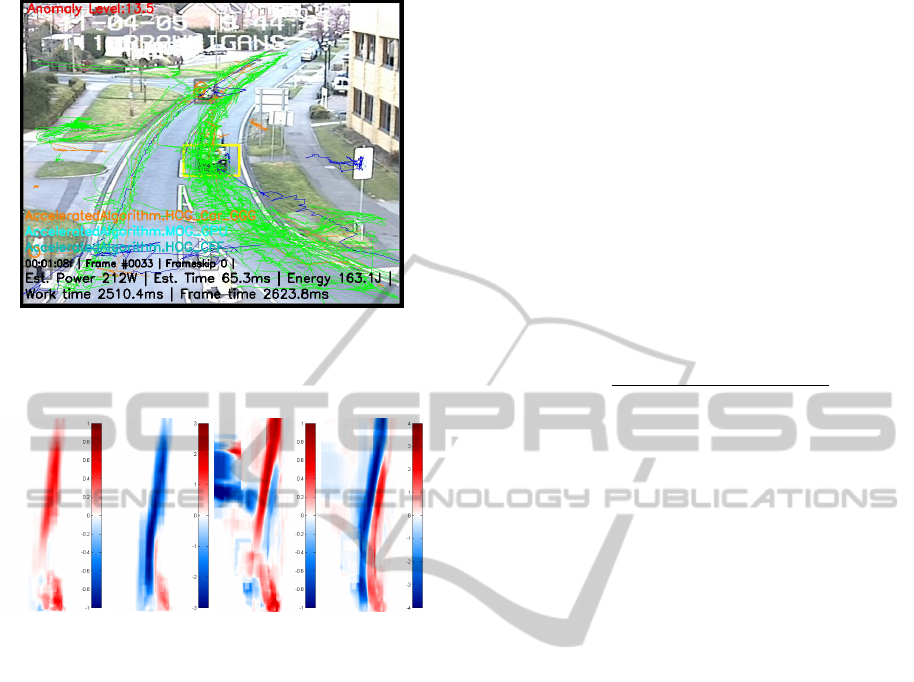
Figure 10: Trajectory clustering via learned object clus-
ters, re-projected onto camera plane. Green, blue and or-
ange tracks represent cars, pedestrians and undetermined
(motion-only) objects respectively.
(a) v
x,ped
(b) v
y,ped
(c) v
x,car
(d) v
y,car
Figure 11: Ground-plane motion intensity maps built us-
ing movement from different object classes in PV3. In (d),
on-road vertical motion away from (blue) and toward the
camera (red) is distinct and clearly defined. Velocity scale
is in pixels per frame.
about the normal or most common actions within the
scene (Robertson and Letham, 2012). Position and
motion information can capture various examples of
anomalous behaviour: for example stationary objects
in an unusual location, or vehicles moving the wrong
way down a street. Unsupervised learning based on
the output of the object classifiers during training se-
quences was used to learn scene context.
Type-specific information about object presence
at different locations in the base plane was captured
by recording the per-pixel location of each base-
transformed bounding box. Average per-pixel veloc-
ity ¯v in x− and y−directions was obtained from the
object trackers. For an object at base plane location
(x ...x
0
, y ...y
0
) with x−velocity v
x
and update rate
α = 0.0002,
¯v
(x...x
0
, y...y
0
)
= (1 −α) ¯v
(x...x
0
, y...y
0
)
+ αv. (2)
This is shown in 11. For most conceivable traffic ac-
tions, presence and motion information is appropri-
ate; however, this fails to capture more complex in-
teractions between people. We therefore focus on be-
haviour involving vehicles.
2.8 Anomaly Detection
Based on 2.7 and 2.6 we can define an anomalous ob-
ject as one which is present in an unexpected area, or
one which is present in an expected area but moves
in an unexpected direction or at an unexpected speed.
A Bayesian framework is used to determine if an ob-
ject’s velocity in the x and y directions should be con-
sidered anomalous, based on the difference between
it and the known average velocity ¯v in that region. We
define the probability of an anomaly at a given pixel
p(A|D), given detection of an object at that pixel:
p(A|D) =
p(D|A)p(A)
p(D|A)p(A) + p(D|
¯
A)p(
¯
A)
, (3)
where the prior probability of an anomaly anywhere
in the image, p(A), is set to a constant value. p(D|A),
the likelihood of detecting an event at any pixel in the
presence of an anomaly, is constant (i.e. we assume
that an anomaly can occur with equal probability any-
where within the image), and p(
¯
A) = 1 − p(A).
p(D|
¯
A) is a measure based on the learned values
for ¯v
x
or ¯v
y
. It expresses the similarity of the observed
motion to mean motion at that pixel, and returns val-
ues between (0.01,0.99). These are based on the dis-
tance between, and relative magnitudes of, v and ¯v:
d
v
=
sgn( ¯v)max(C| ¯v|,| ¯v| +C), if sgn( ¯v)
== sgn(v)
&|v| > | ¯v|
sgn( ¯v)min(−| ¯v|/2,| ¯v| −c), otherwise.
(4)
Here, C and c are forward and reverse-directional con-
stants. d
v
is then used to obtain a linear equation for v,
with a gradient of a = (0.01 − 0.99)/(d
v
− ¯v). Finally,
b is obtained in a similar manner, and v is projected
onto this line to obtain a per-pixel likelihood that v is
not anomalous:
y = av +b , (5)
p(D|
¯
A) = max(0.01,min(0.99,y)). (6)
3 now gives an object anomaly measure UO
x
. This is
repeated for y−velocity data to obtain U O
y
.
This is combined with UC, an abnormality mea-
sure for the cluster linked to that object. When a
trajectory moves from one cluster to one of its chil-
dren, leaves the field of view, or is lost, the number
of transits through that cluster is incremented. For
any trajectory T matched to a cluster C
p
with chil-
dren C
c1
and C
c2
, the number of trajectory transitions
Event-drivenDynamicPlatformSelectionforPower-awareReal-timeAnomalyDetectioninVideo
59

between C
p
and all C
c
is also logged, updating a fre-
quency distribution between C
c1
and C
c2
. These two
metrics (cluster transits and frequency distributions of
parent–to–child trajectory transitions) allow anoma-
lous trajectories to be identified. If C
i
is a root node,
UC(C
i
) = (1 +transits(C
i
))
−1
. Otherwise if C
i
is one
of n child nodes of C
p
,
UC(C
i
) = 1 −
transitions(C
p
→ C
i
)
n
∑
j=1
(transitions(C
p
→ C
j
))
. (7)
An overall anomaly measure U
i
for an object i
with age τ is then obtained:
U
i
= w
o
Σ
τ
i
1
UO
x
τ
i
+ w
o
Σ
τ
i
1
UO
y
τ
i
+ w
c
UC
i
, (8)
and U
max
is updated via U
max
= max(U
max
,U
i
). The
UO measures are running averages over τ. An object
has to appear as anomalous for a time threshold t
A
before affecting U
max
. All w are set to 10, with the
anomaly detection threshold set at 15; two detectors
are thus required to register an object as anomalous
before it is logged.
3 DYNAMIC MAPPING
The mapping mechanism selects algorithm imple-
mentations used to process the next frame. This runs
every time a frame is processed, allowing selection of
a new set of implementations M in response to chang-
ing scene characteristics. M can be any combination
of paths through the algorithms in 4; 1 shows system
power vs. time for all such combinations. Ten cred-
its are allocated between the three priorities P used to
influence the selection of M: power consumption w
p
,
processing time w
t
and detection accuracy w
ε
. Here
we assume that a higher level of anomaly in the scene
should be responded to with increased processing re-
sources to obtain more information about the scene
in a timely fashion, with fewer dropped frames, and
at the expense of lower power consumption. Con-
versely, frames with low or zero anomaly levels cause
power consumption to be scaled back, at the expense
of accuracy and processing time. Realtime process-
ing is then maintained by dropping a greater number
of frames. Prioritisation could be either manual or au-
tomatic. When automatic prioritisation was used, (i.e.
the system was allowed to respond to scene events
by changing its mapping) the speed priority was in-
creased to maximum when U
max
≥ 15. A level of
hysteresis was built in by maximising the power pri-
ority when U
max
< 12. After every processed frame,
Table 2: Performance characteristics (Processing Time
(ms), System Power (W) and Detection Accuracy (log-
average miss rate (%))) for various algorithm implementa-
tions on 770 × 578 video. Baseline power consumption was
147W .
Algo. Impl. Time Power Accuracy
(ms) (W) (%)
HOG ggg 17.6 229 52
(PED) cff 23.0 190 62
gff 27.5 186 61
gfg 39.0 200 59
cfc 117.3 187 59
ccc 282.0 191 53
HOG ggg 34.3 229 89
(CAR) cfc 175.6 189 94
gfg 60.0 200 92
ccc 318.0 194 89
MOG GPU 8.1 202 N/A
if t
process
> FPS
−1
, then dt
process
× FPSe frames are
skipped to regain a realtime rate.
Once a list of candidate algorithms (HOG-PED,
HOG-CAR and MOG) and a set of performance pri-
orities is generated, implementation mapping is run.
This uses performance data for each algorithm imple-
mentation, shown individually for all algorithms in 2.
Exhaustive search is used to generate and evaluate all
possible mappings, with a cost function:
C
i
= w
p
P
i
+ w
t
t
i
+ w
ε
ε
i
, (9)
where all w are controlled by P. Estimated power,
runtime and accuracy is also generated at this point.
The lowest-cost mapped algorithms are then run se-
quentially to process the next frame and generate de-
tections.
4 EVALUATION METHODS
Clusters and heatmaps were initialised by training on
two 20-minute daylight clips from the i-LIDS train-
ing set. Each test sequence was then processed in ap-
proximately real time using this data. Clusters and
heatmaps were not updated between test videos. The
homography matrices used to register each video onto
the base plane were obtained manually. Tests were
run three times and referred to as follows, using the
prioritisation settings described in 3:
speed speed prioritised, auto prioritisation off;
power power prioritised, auto prioritisation off;
auto anomaly-controlled auto prioritisation on.
For each run, all anomalous events (defined as ob-
jects having U > 15 for more than a fixed time limit
t
A
= 10 or 15 seconds) were logged and compared
VISAPP2014-InternationalConferenceonComputerVisionTheoryandApplications
60
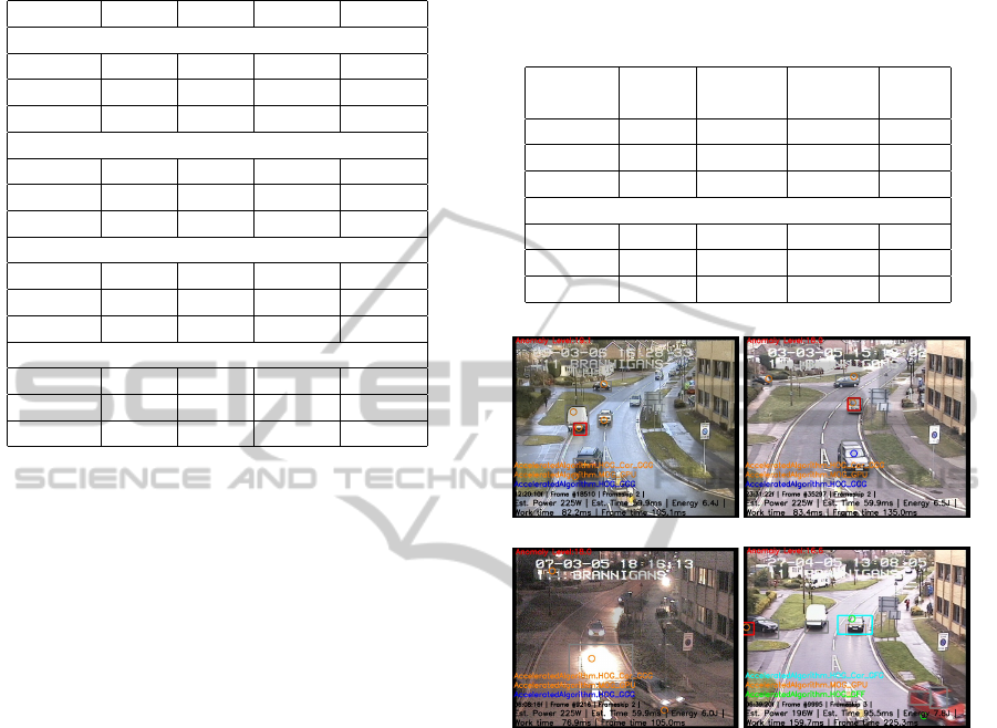
Table 3: Detection performance (precision and recall) for
parked vehicle events on i-LIDS PV3. F
1
-scores are shown
for operational awareness (OA) and event logging (EL).
Priority p r F
1,OA
F
1,ER
for t
A
= 10 seconds
power 0.083 0.133 0.0957 0.1317
speed 0.105 0.194 0.1254 0.1913
auto 0.102 0.194 0.1226 0.1912
for t
A
= 10 seconds, daylight only
power 0.121 0.148 0.1294 0.1475
speed 0.130 0.214 0.1510 0.2118
auto 0.125 0.214 0.1466 0.2115
for t
A
= 15 seconds
power 0.118 0.065 0.0910 0.0652
speed 0.381 0.258 0.3259 0.2594
auto 0.222 0.133 0.1797 0.1342
for t
A
= 15 seconds, daylight only
power 0.167 0.065 0.1067 0.0652
speed 0.500 0.258 0.3752 0.2601
auto 0.286 0.133 0.2030 0.1345
with ground-truth data. Power consumption for one
frame was estimated by averaging the energy used
to process each implementation over runtime for that
frame. Average power consumption over a sequence
of frames was obtained in the same manner.
A modified version of the i-LIDS criteria was used
to evaluate detection performance. Events count as
true positives if they are registered within 10 seconds
of the start of an event. For parked vehicles, i-LIDS
considers the start of the event to be one full minute
after the vehicle is parked, whereas we consider the
start of the event to be when it parks. We may thus
flag events before the timestamp given in the ground
truth data. The time window for matching detections
is thus 70 or 75 seconds long. The i-LIDS criteria
only require a binary alarm signal in the presence of
an anomaly; however, we require anomalous tracks to
be localised to the object causing the anomaly. The
detection in 12(d) is thus incorrect; the white van is
stopped and should be registered as an anomaly, but
the car on the left is flagged instead. This counts as
one false-negative and one false-positive event.
5 RESULTS
i-LIDS uses the F
1
score (F
1
= (α + 1)rp/(r + αp))
for comparing detection performance. α is set at 0.55
for real-time operational awareness (to reduce false-
alarm rate), or 60 for event logging (to allow logging
of almost everything with low precision).
3 shows precision, recall and F
1
scores for all
“parked vehicle” events in the PV3 scenario for t
A
=
Table 4: Processing performance for all prioritisation
modes, showing percentage of frames skipped, ( f skip), pro-
cessing time including (t
f rame
) and excluding overheads
(t
work
) compared to source frame time (t
src
), and mean esti-
mated power above baseline (P
∗
work
). Idle/baseline power is
147W.
Priority f skip t
f rame
/ t
work
/ P
∗
work
(%) t
src
(%) t
src
(%) (W)
power 75.8 125.4 87.9 49.1
speed 59.5 124.3 81.7 72.8
auto 66.5 127.8 83.4 61.9
daylight only
power 75.5 125.4 87.9 49.1
speed 60.1 124.2 82.0 78.4
auto 66.0 122.0 83.4 61.8
(a) TP (b) TP
(c) FN (d) FN, FP
Figure 12: True detections and failure modes of anomaly
detector on i-LIDS PV3. (a), (b): true positives in varying
locations. (c): false negative caused by occlusion. (d) is
treated as a false negative and a false positive as the detector
identifies the car on the left instead of the van parked beside
it.
10 and 15 seconds. Night-time sequences have no
events but still generate a large proportion of false
positives, so this also shows results for daylight-only
(“day” and “dusk” clips) separately.
4 shows performance details for all three prior-
ity modes. The t
f rame
column shows overall execu-
tion time (including overheads) relative to total source
video length. The processing time column does not
include overheads. It assumes that a raw video frame
is already present in memory, and frame-by-frame
video output is not required (i.e. only events are
logged). In this case, the system runs faster than real-
time, with the percentage of skipped frames shown in
the f skip column. The slower power-optimised prior-
ity setting causes more frames to be skipped.
Event-drivenDynamicPlatformSelectionforPower-awareReal-timeAnomalyDetectioninVideo
61
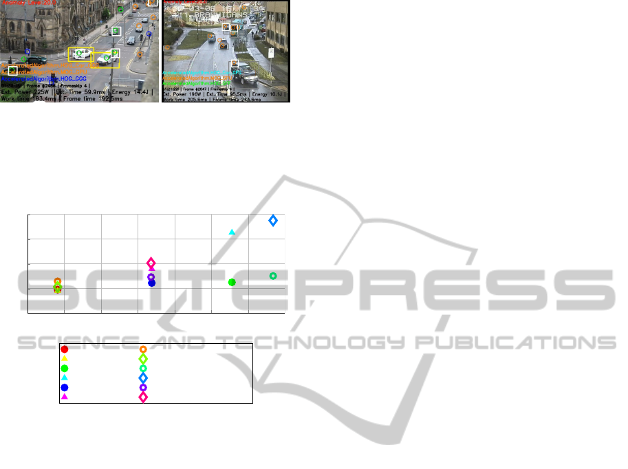
(a) High-quality video (b) i-LIDS video
Figure 13: Dataset quality impacts quality of detections: in
a separate video (a), video quality allows classification of
most objects as either pedestrian (blue circle) or car (green
circle). In i-LIDS, (b), detections often remain as uncate-
gorised motion (orange circle).
45 50 55 60 65
70
75
80
0
0.1
0.2
0.3
0.4
system power consumption above baseline (W)
F
1
-score (α = 0.55)
power, t
A
= 10 sec
power, t
A
= 10 sec, daylight
power, t
A
= 15 sec power, t
A
= 15 sec, daylight
speed, t
A
= 10 sec speed, t
A
= 10 sec, daylight
speed, t
A
= 15 sec speed, t
A
= 15 sec, daylight
auto, t
A
= 10 sec
auto, t
A
= 10 sec, daylight
auto, t
A
= 15 sec auto, t
A
= 15 sec, daylight
Figure 14: F
1
−scores for operational awareness (α = 0.55)
against power consumption, for various time thresholds.
12 shows example detections logged after t
A
sec-
onds. While some true positives are detected (up to
50% in the best case), many false negatives and false
positives are present, and have various causes. False
positive are often caused by the background subtrac-
tor erroneously identifying patches of road as fore-
ground, caused by the need to acquire slow-moving
or waiting traffic in the same region. False nega-
tives are, in general, caused by poor performance of
the object classifiers or background subtractor. Di-
rectly failing to detect partially occluded objects (as
in 12(c)), or stationary, repeated false detections in
regions overlapping the roadside which are gener-
ated during training can both cause anomalies to be
missed. Poorer video quality also reduces detection
accuracy, as shown in 13.
6 DISCUSSION
Given that the system must run in real-time (as we
drop frames to ensure a close-to-realtime rate), the
main tradeoffs available here are accuracy and power;
optimising for time allows more frames to be pro-
cessed, which in combination with the natural in-
creased detection accuracy of the ggg detectors, in-
creases p and r. This is borne out by the data in 3.
The key figures in 4 are mean estimated power
consumption above baseline; there is 29W range in
average power consumption between highest-power
and lowest-power priority settings. When the system
was run with speed prioritised with the FPGA turned
off, power consumption was 208W , or 62W above
baseline. The average power for auto-prioritised
mode with the FPGA on was 61.9W , but this is de-
pendent on the dataset used; datasets with fewer mov-
ing objects would have a lower average power con-
sumption than this. As 14 shows, running the system
in automatic prioritisation mode allows an increase in
accuracy of 10% over the lowest-power option for a
cost of 12W in average power consumption. A further
17% gain in F
1
−score (from auto to speed) costs an
extra 17W above baseline. These results show a clear
relationship between power consumption and overall
detection accuracy.
6.1 Comparison to State-of-the-Art
Some previous work has considered four clips made
publicly available from i-LIDS, known as AVSS and
containing 4 parked-vehicle events, classed as easy,
medium, hard and night. The only work we are aware
of which evaluates the complete i-LIDS dataset is (Al-
biol et al., 2011). Using spatiotemporal maps and
manually-applied lane masks per-clip to denote ar-
eas in which detections are allowed, Albiol et al. are
able to improve significantly on the precision and re-
call figures given above, reaching p− and r−values
of 1.0 for several clips in PV3. They do not provide
performance information but note that they downscale
the images to 240 × 320 to decrease evaluation time.
In their work they discuss the applicability and limi-
tations of background subtractors for detecting slow-
moving and stopped objects, as well as discussing the
same difficulties with the i-LIDS data previously seen
in 13. As in 1, we also consider real-time implemen-
tation and power consumption, with an end goal of a
fully automatic system. Unlike Albiol et al.’s require-
ment for manual operator intervention, we only need
to re-register videos between clips to overcome cam-
era movement, which could be done automatically.
If we only consider our detector accuracy compared
to those of other researchers working on this data,
we cannot improve upon existing results. However,
we are tackling the novel problem of power-aware
anomaly detection rather than offline lane masking,
and any accuracy measurement must be traded against
other characteristics, as 14 shows. The most obvi-
ous way to improve these results would be to use the
VISAPP2014-InternationalConferenceonComputerVisionTheoryandApplications
62

currently best-performing object classifiers, but im-
plementing multiple heterogeneous versions of these
would take prohibitively long to develop.
7 CONCLUSIONS
We have described a real-time system for performing
power-aware anomaly detection in video, and applied
it to the problem of parked vehicle detection. We are
able to select between various algorithm implementa-
tions based on the overall object anomaly level seen
in the image, and update this selection every frame.
Doing this allows us to dynamically trade off power
consumption against detection accuracy, and shows
benefits when compared to fixed power- and speed-
optimised versions. Although the accuracy of our de-
tection algorithms (HOG) alone is no longer state-of-
the-art, future improvements include introduction of
more advanced object classifiers (such as (Benenson
and Mathias, 2012)) and a move to a mobile chipset,
which would reduce idle power consumption while
maintaining both speed and accuracy, with the trade-
off of increased development time.
ACKNOWLEDGEMENTS
We gratefully acknowledge the work done by Scott
Robson at Thales Optronics for his FPGA implemen-
tation of the histogram generator for the CAR-HOG
detector.
This work was supported by the Institute for System
Level Integration, Thales Optronics, the Engineer-
ing and Physical Sciences Research Council (EPSRC)
Grant number EP/J015180/1 and the MOD Univer-
sity Defence Research Collaboration in Signal Pro-
cessing.
REFERENCES
Albiol, A., Sanchis, L., Albiol, A., and Mossi, J. M. (2011).
Detection of Parked Vehicles Using Spatiotemporal
Maps. IEEE Transactions on Intelligent Transporta-
tion Systems, 12(4):1277–1291.
Bacon, D., Rabbah, R., and Shukla, S. (2013). FPGA Pro-
gramming for the Masses. Queue, 11(2):40.
Benenson, R. and Mathias, M. (2012). Pedestrian detection
at 100 frames per second. In Computer Vision and
Pattern Recognition (CVPR), 2012 IEEE Conference
on, pages 2903–2910.
Blair, C., Robertson, N. M., and Hume, D. (2013). Char-
acterising a Heterogeneous System for Person Detec-
tion in Video using Histograms of Oriented Gradi-
ents: Power vs. Speed vs. Accuracy. IEEE Journal
on Emerging and Selected Topics in Circuits and Sys-
tems, 3(2):236–247.
Bouganis, C.-S., Park, S.-B., Constantinides, G. A., and
Cheung, P. Y. K. (2009). Synthesis and Optimization
of 2D Filter Designs for Heterogeneous FPGAs. ACM
Transactions on Reconfigurable Technology and Sys-
tems, 1(4):1–28.
Cope, B., Cheung, P. Y., Luk, W., and Howes, L. (2010).
Performance Comparison of Graphics Processors to
Reconfigurable Logic: A Case Study. IEEE Transac-
tions on Computers, 59(4):433–448.
Dalal, N. (2006). Finding People in Images and
Videos. PhD Thesis, Institut National Polytechnique
de Grenoble / INRIA Grenoble.
Dalal, N. and Triggs, B. (2005). Histograms of oriented
gradients for human detection. In Computer Vision
and Pattern Recognition, 2005. CVPR 2005., pages
886– 893. IEEE Computer Society.
Everingham, M., Gool, L., Williams, C. K. I., Winn, J.,
and Zisserman, A. (2009). The Pascal Visual Object
Classes (VOC) Challenge. International Journal of
Computer Vision, 88(2):303–338.
Home Office Centre for Applied Science and Technology
(2011). Imagery Library for Intelligent Detection Sys-
tems (I-LIDS) User Guide. UK Home Office, 4.9 edi-
tion.
Piciarelli, C. and Foresti, G. (2006). On-line trajectory clus-
tering for anomalous events detection. Pattern Recog-
nition Letters, 27(15):1835–1842.
Robertson, N. and Letham, J. (2012). Contextual Person
Detection in Outdoor Scenes. In Proc. European Con-
ference on Signal Processing (EUSIPCO 2012).
Yu, Y. and Prasanna, V. (2002). Power-aware resource al-
location for independent tasks in heterogeneous real-
time systems. In Ninth International Conference on
Parallel and Distributed Systems, 2002. Proceedings.,
pages 341–348. IEEE Comput. Soc.
Zivkovic, Z. (2004). Improved adaptive Gaussian mixture
model for background subtraction. In Proceedings of
the 17th International Conference on Pattern Recog-
nition, 2004. ICPR 2004., volume 2, pages 28–31.
IEEE.
Event-drivenDynamicPlatformSelectionforPower-awareReal-timeAnomalyDetectioninVideo
63
