Visualization of Remote Sensing Imagery by Sequential Dimensionality

Reduction on Graphics Processing Unit

Safa A. Najim

1,2

and Ik Soo Lim

School of Computer Science, Bangor University, Bangor, Gwynedd, U.K.

Computer Science Dept., Science College, Basrah University, Basrah, Iraq

Keywords:

Visualization, Dimensionality Reduction, Remote Sensing Imagery, Graphics Processing Unit (GPU).

Abstract:

This paper introduces a new technique called Sequential Dimensionality Reduction (SDR), to visualize remote

sensing imagery. The DR methods are introduced to project directly the high dimensional dataset into a low

dimension space. Although they work very well when original dimensions are small, their visualizations are

not efﬁcient enough with large input dimensions. Unlike DR, SDR redeﬁnes the problem of DR as a sequence

of multiple dimensionality reduction problems, each of which reduces the dimensionality by a small amount.

The SDR can be considered as a generalized idea which can be applied to any method, and the stochastic

proximity embedding (SPE) method is chosen in this paper because its speed and efﬁciency compared to other

methods. The superiority of SDR over DR is demonstrated experimentally. Moreover, as most DR methods

also employ DR ideas in their projection, the performance of SDR and 20 DR methods are compared, and the

superiority of the proposed method in both correlation and stress is shown. Graphics processing unit (GPU)

is the best way to speed up the SDR method, where the speed of execution has been increased by 74 times in

comparison to when it was run on CPU.

1 INTRODUCTION

Visualization of high dimensional dataset is widely

used in many ﬁelds including remote sensing imagery,

biology, computer vision, and computer graphics in

order to analyze them (Blum and Liu, 2006). The di-

mensionality reduction (DR) method is one of the best

strategies used in this matter by projecting high di-

mensional space onto lower dimensional space where

they can be visualized directly. The colour of each

pixel in the visualization is a compendium of infor-

mation in the original data in which their most salient

features are captured (Kaski and Peltonen, 2011) (Pel-

tonen, 2009).

Nonlinear projection has received signiﬁcant at-

tention in modern DR methods due to its intrinsic

ability to generate visualization with respect to prox-

imity between instances of data (Lawrence et al.,

2011) (Mokbel et al., 2013). They have the advan-

tage of perfect colours, which in turn often have clear

meanings. In contrast, linear projection generates

poor and worst interpretations of large datasets (Tyo

et al., 2003) (Steyvers, 2002). The task of DR is vi-

sualization of neighbourhood or proximity relation-

ships within a high dimensional space. The visualiza-

tion should allow the user to retrieve the neighbour-

ing data points in original space. Perfect neighbour-

hood preserving is usually not possible, and applying

the DR method makes two kinds of errors: decreas-

ing continuity neighbourhood, and increasing false

neighbourhood (Lespinats and Aupetit, 2011). In

false neighbourhoods, a large distance between origi-

nal data points becomes a small distance in the lower

dimensional space, which have the same colour in vi-

sualization, as in Figure 1. Thus, the colours of vi-

sualization have no meaning because the straightfor-

ward relationship with original high dimension space

is lost (Bachmann et al., 2005).

Due to the difference between the topological

structure of data points in high dimension space with

the topological structure of projected space, it is difﬁ-

cult to preserve the neighbourhood relations between

data points. Eventually, the way of applying DR it-

self is not perfect. Loss of any neighbour point could

lead to an increase in the the amount of error be-

cause the missing neighbour point will occupy a place

of another point in the lower space. Therefore, the

amount of error could be growing explosively when

increasing the false neighbourhood. Overlap between

points is the dominate thing when direct projection

Najim S. and Lim I..

Visualization of Remote Sensing Imagery by Sequential Dimensionality Reduction on Graphics Processing Unit.

DOI: 10.5220/0004737500710079

In Proceedings of the 5th International Conference on Information Visualization Theory and Applications (IVAPP-2014), pages 71-79

ISBN: 978-989-758-005-5

 2014 SCITEPRESS (Science and Technology Publications, Lda.)

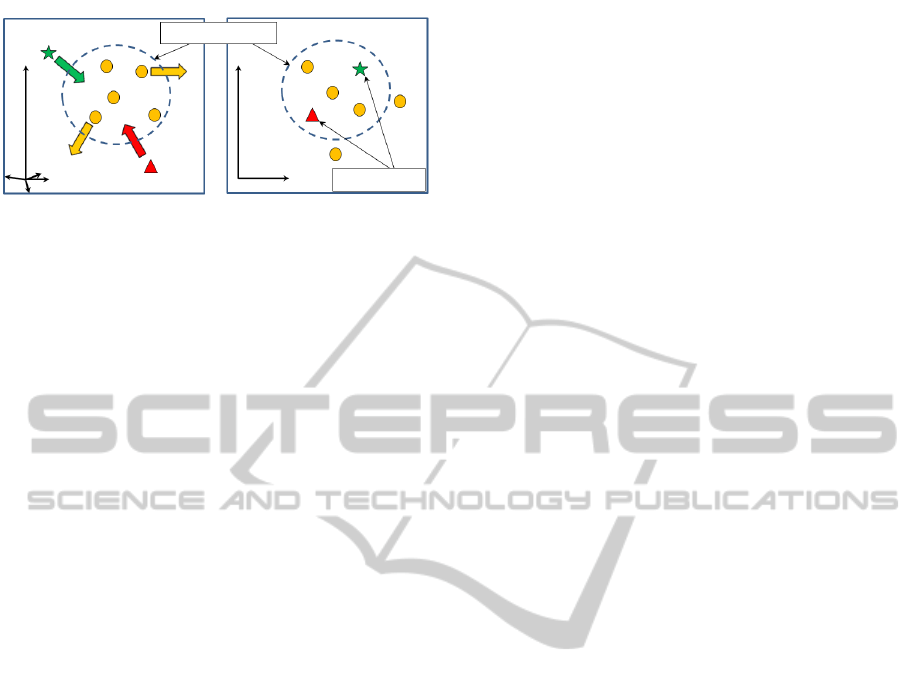
High dimensional space Low dimensional space

Local neighborhood

False neighbors

Figure 1: DR might cause the points which are outside lo-

cal neighborhood in high dimension space to be inside lo-

cal neighborhood in low dimension space. These points are

called false neighborhood.

from high dimension space to lower dimension space

is still used.

This work proposes a novel DR method, called

Sequential Dimensionality Reduction (SDR), which

is used to optimize the quality of visualization as a

sequence of multiple dimensionality reduction prob-

lems, each of which reduces the dimensionality by a

small amount. In contrast to the DR method, SDR

preserves the neighbourhood relations between data

points of two reduced consecutive spaces. Thus, false

neighbourhoods are reduced as much as possible.

This paper is organized as follows: Section 2 gives

some ideas about related works. In section 3, method-

ology of proposed method is explained. Experimental

results are dominated in section 4. Finally, the conclu-

sion is drawn in section 5.

2 RELATED WORK

2.1 Visualization by DR

The technique of DR is useful to visualize and analyse

that large volume of data. For a set of n input points

X ∈ ℜ

, φ(X) is used to project the D dimensional

data points (x

∈ X) to d dimensional data points (y

∈

Y ):

φ : ℜ

→ ℜ

(1)

7→ y

∀ 1 ≤ i ≤ n (2)

In equation 1, φ attempts to approximate

the input pairwise distance r(x

) with their

corresponding in projected space d(y

), i.e,

r(x

) ≈ d(y

) ∀ 1 ≤ i ≤ n to project X’s

data point correctly in Y space. Loss of preserv-

ing neighborhood relations should be minimized, i.e.

Ξ(φ(X)) ≈ X, where Ξ : ℜ

→ ℜ

. Thus, DR at-

tempts to minimize Equation 3.

Stress(φ) =

∑

i, j=1

i j

− d

i j

)

(3)

where r

i j

= ||x

− x

|| and d

i j

= ||y

− y

||.

The variety of strategies have resulted in the de-

velopment of many different DR methods. Linear and

nonlinear DR methods are the best examples to de-

scribe them.

Linear projection: Principle components analysis

(PCA) uses orthogonal linear combination to ﬁnd lin-

ear transformation space of data set. Because of its

simplicity, it is used for data visualization (Jolliffe,

2002). Other visualization methods aim to preserve

distances, such as multidimensional scaling (MDS)

(Borg and Groenen, 1997). It computes distance ma-

trix among points by computing pairwise Euclidean

distances. PCA and MDS fail to ﬁnd satisfactory low

dimension representation of nonlinear data.

Nonlinear projection: Modern DR methods usually

use nonlinear projections to project the data into low

dimensions. Kernel PCA (Shawe-Taylor and Cris-

tianini, 2004) is a nonlinear version of PCA, and iso-

metric feature mapping (Isomap) (Tenenbaum et al.,

2000) uses geodesic distance rather than Euclidean

distance in MDS. Other methods use local linear re-

lationships to measure the local structure, as in lo-

cal linear embedding (LLE) (Roweis and Saul, 2000),

maximum variance unfolding (MVU) preserves di-

rect neighbours while unfolding data (Weinberger and

Saul, 2006), and laplacian eigenmaps (Belkin and

Niyogi, 2002) take a more principled technique by

referring to the spectral properties of the resulting

dissimilarity matrix. Some methods, like stochas-

tic neighbor embedding (SNE) (Bunte et al., 2012),

t-distributed stochastic neighbor embedding (t-SNE)

(Maaten and Hinton, 2008) and neighborhood re-

trieval visualizer (NeRV) (Venna et al., 2010), attempt

to match probability distributions induced by the pair-

wise data dissimilarities in the high dimensional space

and low dimension space, respectively. Stochastic

proximity embedding (SPE) proceeds by calculating

Euclidean distance for global neighbourhood points

within ﬁxed radius (Agraﬁotis et al., 2010). It is an

enormous step in computational efﬁciency over MDS,

and faster than Isomap.

Many solutions to visualize dataset in DR have

been proposed (Maaten et al., 2009), but fewer so-

lutions exist to overcome false neighbourhoods. The

preserving neighbourhood relations by DR remains a

matter of controversy between researchers.

IVAPP2014-InternationalConferenceonInformationVisualizationTheoryandApplications

2.2 Quality of Visualization

When measuring the quality of visualization for a

given dataset it is important to know which DR

method is best suited for the task at hand. Further-

more, humans cannot compare the quality of a given

visualization with original data by visual inspection

due to its high dimensionality. Thus, the best formal

measurements should evaluate the amount of preserv-

ing neighbourhood colour distances in the visualiza-

tion with their corresponding in original data. Cor-

relation (ρ) and residual variance (RV ) are the well-

known methods used in this matter. If we suppose X

is a vector of all pairwise distance of the data points in

original space and Y is a vector of their corresponding

pairwise colour distances in visualization, then their

deﬁnitions are:

Residual Variance (RV ) is a function used to com-

pute the standard error of difference between visual-

ization and original space (Tenenbaum et al., 2000). It

calculates the sum of squares of differences between

original data point distances and projected colour dis-

tances, as in equation 4.

RV =

∑

(X −Y )

N − 2

(4)

where N is length of X vector. By Equation 4, small

stress value indicates that visualization has very little

error and higher efﬁciency.

In Correlation function (γ), the linear correlation be-

tween original input distances and colour distances

in visualization is computed (Mignotte, 2012). The

value of correlation is equal to 1 when all distances

between two vectors are perfect preserved with posi-

tive slope. In the other hand, the value equal to -1 if

the two vectors have prefect linear relationship with

negative slope. The correlation is deﬁned by:

γ =

Y /|X| − X Y

(5)

where |X| is the length of X, and X and σ

are the

mean and standard deviation of X, respectively.

2.3 Visualization of Remote Scening

Imagery

Remote scening imagery is a well-known technique

to observe the earth and urban scenes by producing a

large number of spectral bands (Smith, 2012). How-

ever, the challenge is how to display the abundant in-

formation contained in these images in a more inter-

active and easy analysed way, such as in a 3-D im-

age cube. Due to the difﬁculty of using these huge

bands, several DR methods are produced to overcome

this problem by ﬁnding the best relationships among

colour values in three colour channels after applying

complex formulas to shrink the huge original space.

DR provides a good way to visualize hyperspectral

imagery by generating its colour image (Bachmann

et al., 2005) (Mignotte, 2012).

2.4 Graphics Processing Unit (GPU)

Recently, the processing power and memory band-

width of a new generation of graphics card

have emerged as a powerful computation platform

(Sanders and Kandrot, 2011). GPU has many pro-

grammable processors working in a highly parallel

style. Compute Uniﬁed Device Architecture (CUDA)

is the hardware and software NVIDIA parallel com-

puting architecture that is Integrated Development

Environment (IDE) such as Microsoft C++ Visual

Studio, to write the CUDA C++ program. It has two

types of functions: host and kernel. Host functions are

run in CPU to execute the sequential codes, and ker-

nel functions are responsible for the execution of the

parallel instructions inside GPU. Kernel function can-

not be called directly where it should be called from

host function. The GPU consists of a set of small

processing units (called threads) which are grouped

into blocks. Each thread has a small private memory,

and each block has memory to share their threads to-

gether. In addition, all GPU’s threads can access CPU

memory in a memory portion called global memory.

Threads in a block synchronize their cooperation in

accessing shared memory. Because the CPU consists

of a few cores for executing serial processing, CPU

and GPU construct a power combination which is de-

signed for parallel and serial performances.

3 METHODOLOGY:

SEQUENTIAL DR

The goal of the proposed method is to solve the DR

by ﬁnding a representation of N points in d space,

where its neighbourhood relationships are preserved

with their corresponding relations in original space.

To do that, we redeﬁne the problem of DR as a se-

quence of multiple DR problems, each of which re-

duces the dimensionality by a small amount. We call

this Sequential Dimensionality Reduction (SDR).

More speciﬁcally, given X = x

,..., x

be a

data with instances x

∈ ℜ

. SDR attempts to do the

VisualizationofRemoteSensingImagerybySequentialDimensionalityReductiononGraphicsProcessingUnit

Local

neighborhoods

D−2

D−1

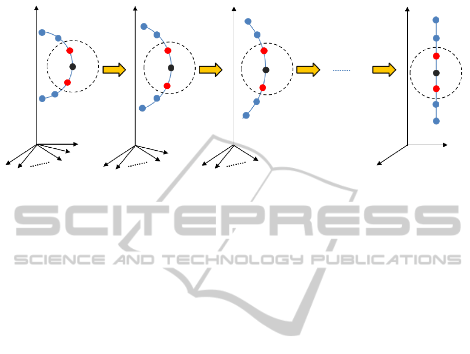
Figure 2: SDR redeﬁnes the problem of DR as a sequence of multiple DR problems, each of which reduces the dimension-

ality by a small amount. When amount of dimensionality reduction is equal to 1, the amount of losing information when

transforming from v space to v − 1 space is very few, where v ∈ {D,D −1, D − 2,..., d +1}. The neighborhoods of point p

preserved in D − 1, D − 2, ..., and d spaces.

transformation in equation 6.

G : ℜ

−→ ℜ

D−1∗S

−→ ℜ

D−2∗S

−→ ℜ

D−3∗S

−→ ℜ

(6)

where D >> d, and S is the step of dimensionality re-

duction can be in the range [1, D − 1].

The transformation (G

) attempts to project N points

of (D − (i − 1) ∗ S) space into (D − i ∗ S) space. The

transformation between two spaces is reasonably as

close as possible because of the similarity of dimen-

sionality between two spaces. Thus, the problem for

(D − i ∗ S) space is solved. Efﬁciency of transforma-

tion permits to recursively apply it until the target di-

mension is obtained. Therefore, the neighbourhood

relations between original points are kept carefully

through a sequence of transformations until it obtains

d space.

Figure 2 shows the general idea of the SDR when

S = 1. The point p

in the v space is able to preserve

its neighbour relationships when it is projected to the

v −1 space. Thus, the amount of false neighbourhood

when G

: ℜ

→ ℜ

v−1

is very small because the dif-

ference between the two spaces is just one dimension.

A complete transformation from D space to d spaces

is obtained by applying equation 6.

The point which should be discussed is how to

choose S. As we deﬁned before, S can be in the range

[1, D − 1]. For higher efﬁciency S = 1 , where the

intermediate transformation problem will be between

very close topology spaces. The error is minimized,

and the problem is deﬁned as a D − 1 DR problem.

The efﬁciency is reduced when S > 1, and the worst

case when S = D −1 which is deﬁned as one DR prob-

lem.

SDR accepts as input set of N points in D space, a

transformation function G, and the amount of dimen-

sionality reduction S. d is the dimension of lower

space which should be given. SDR algorithm recur-

sively reduces the dimensionality of a space until ob-

taining the target space, and the following steps de-

scribe that:

1. let v = D.

2. if v is equal to d

{Stop}

3. let v −S is the dimension of the next lower space.

4. N points of v space is projected in v − S space

by applying G : ℜ

→ ℜ

v−S

5. let v = v − S, and go to step 2.

Brieﬂy, SDR put the projected points in the cor-

rect location in low dimension space, which leads to

a reduction in the amount of error and an increase in

the degree of compliance with original space. The ef-

ﬁciency of SDR is clearer when input dimension is

very high and target dimension is very low. We chose

the SPE method to be used with the SDR idea (to gen-

erate SSPE) because SPE has more advantages than

other methods, as we will see in next subsection.

The length of the execution time is one of the lim-

itations that is encountered with the SDR, therefore,

using GPU is the most appropriate way to overcome

this problem.

3.1 SPE

SPE is a nonlinear method and proceeds by calcu-

lating Euclidean distance for global neighbourhood

IVAPP2014-InternationalConferenceonInformationVisualizationTheoryandApplications

points within a ﬁxed radius (r

) (Agraﬁotis et al.,

2010). SPE is an enormous step forward in compu-

tational efﬁciency over MDS, and faster than Isomap.

SPE is used in different applications and has suc-

ceeded in getting satisfactory results (Ameer and Ja-

cob, 2012). The objective of SPE is to ﬁnd a represen-

tation which has point’s distances which are identical

to their corresponding distances in high dimensional

space. The method starts by selecting a random point

from the original data, in time (t

) to be projected in

the low dimension space. Projection points means the

withdrawal of the neighbourhood points within ﬁxed

radius (r

Projected space starts with initial coordinates, and

it is updated iteratively by placing y

onto the pro-

jected space in such a way that their euclidean dis-

tance (d

i j

= ||y

− y

||) is closed to the corresponding

distance (r

i j

= ||x

− x

||) in original high dimensions

space. Thus, SPE minimizes Equation 3. The points

in projected space are updated according to following

constraint:

i f (r

i j

≤ r

) or ((r

i j

> r

) and (d

i j

< r

i j

))

← x

+ λ(t

)

i j

− d

i j

+ ε

(7)

where λ(t

) is learning rate at t

time, and ε a tiny

number used to avoid division by zero (we used

ε = 1x10

−8

SDR with SPE generates a new method, which we

call SSPE, which uses the idea of SDR and SPE’s

objective function. While SPE objective function is

proved by its minimized function (Agraﬁotis et al.,

2010) when transforming D space to d space (D >>

d), SSPE will be minimizing for the same reasons be-

cause nothing is changed in relation between D and d

spaces.

4 EXPERIMENTAL RESULTS

In this section, the SDR and DR methods are evalu-

ated in quantitative and qualitative manners. The per-

formance of the proposed method is analysed using

remote sensing imagery dataset. The SDR idea is im-

plemented on SPE, which is called SSPE, and com-

pared with tradition SPE. The comparison SDR with

20 DR methods is also included, and Table 1 shows

information about those methods.

The implementations were carried out on a com-

puter which has Intel(R) Cores(TM) i5 CPU M520

2.4Ghz and NVIDIA GeForce GTX 280 with buffer

size 1024 MBytes. Matlab and Microsoft Visual Stu-

dio C++ 2008 Professional Edition with CUDA were

Table 1: Methods employed in comparison. The ﬁrst col-

umn contains the name of methods, second column shows

the type (T) of method (linear (L) or nonlinear (NL)), third

column shows the source of reference and the symbol X

in the fourth column indicates the original codes (O) have

been used.

Method T Source O

PCA L (Jolliffe, 2002) X

CCA L (Demartines and Hrault,

1997)

CDA NL (Lee et al., 2004) X

Factor analysis NL (Darlington, 1999)

Fast MVU NL (Weinberger and Saul,

2006)

Hessian LLE NL (Donoho and Grimes,

2005)

Isomap NL (Tenenbaum et al.,

2000)

Kernel PCA NL (Shawe-Taylor and

Cristianini, 2004)

Laplacian NL (Belkin and Niyogi,

2002)

LDA L (Duda et al., 2001)

LLC NL (Shi and Malik, 2000)

LLE NL (Roweis and Saul,

2000)

LLTSA NL (Zhang et al., 2007)

LPP L (Zhi and Ruan, 2008)

LTSA NL (Zhang and Zha, 2004)

NPE NL (He et al., 2005) X

Prob PCA NL (Tipping and Bishop,

1999)

SPE NL (Agraﬁotis et al., 2010) X

SNE NL (Bunte et al., 2012) X

tSNE NL (Maaten and Hinton,

2008)

used to write the codes. We used the AVIRIS Moffet

Field data set from the southern end of San Francisco

Bay, California, done in 1997 (AVIRIS, 2013). Be-

cause some methods cannot work with large dataset,

we divided this dataset into small regions, each one

with 300x300x224 pixels, and we selected 3 regions

of them.

Table 2 shows SSPE achieves more accurate cor-

relation and stress values. For all regions, the correla-

tion values by our proposed method are highest, and

same is also true for stress values in which it has given

lesser values.

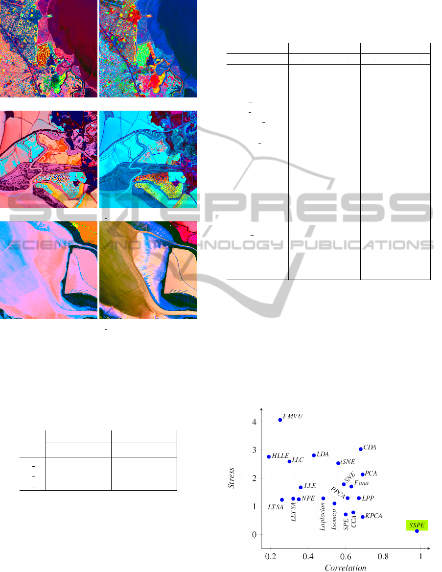
To compare the SDR and DR methods in a qualita-

tive manner, the visualizations of SPE and SSPE are

compared, as in the Figure 3. The performances of

the proposed method in previous table are conformed

here. For example, in the visualizations of regions

1, 2, and 3, SSPEs’ visualizations show more details,

VisualizationofRemoteSensingImagerybySequentialDimensionalityReductiononGraphicsProcessingUnit

(a) R 1

(b) R 2

Figure 3: Visualizations of regions 1, 2, and 3 by using

SPE (in left side) and SSPE (on the right side). The SSPE’s

visualizations in all regions show more details than SPE’s

visualizations.

Table 2: Results of comparison the SDR method (repre-

sented by SSPE), when S = 1, with the DR method (repre-

sented by SPE). The proposed method got the highest cor-

relation and less stress values in all regions.

Correlation Stress

SPE SSPE SPE SSPE

R 1 0.696 0.998 0.033 0.022

R 2 0.641 0.966 1.504 0.261

R 3 0.813 0.989 1.102 0.131

which cannot be recognized by SPE. Let us explain

that with this example, in the top right corner of the vi-

sualization of region 3, the area is incorrectly visual-

ized by SPE, but it has been well visualized by SSPE.

This is due to the fact the number of false colours are

higher than true colours in SPE’s visualization, which

effected the accuracy of that area. The same situation

occurs in the remaining regions where the proposed

method was proven to show the correct colours.

The results of comparisons of the proposed

Table 3: Correlation and stress values of comparisons

among 21 methods for three regions. SSPE , when S = 1,

is the best in all cases, where it has higher correlation and

lesser stress values than other methods.

Correlation Stress

Method R 1 R 2 R 3 R 1 R 2 R 3

PCA 0.69 0.67 0.70 0.71 1.37 4.30

CCA 0.86 0.52 0.53 0.11 1.27 0.97

CDA 0.55 0.75 0.75 5.70 1.18 2.21

Fact analysis 0.83 0.42 0.65 0.90 3.88 0.32

Fast MVU 0.34 0.40 0.00 3.50 5.68 3.03

Hessian LLE 0.27 0.29 0.00 0.72 5.43 2.13

Isomap 0.53 0.65 0.45 0.72 1.13 1.44

Kernel PCA 0.70 0.77 0.59 0.44 0.96 0.46

Laplacian 0.24 0.62 0.58 1.08 1.77 0.97

LDA 0.26 0.43 0.59 1.86 1.04 5.53

LLC 0.24 0.34 0.32 2.42 1.84 3.52

LLE 0.33 0.37 0.37 0.71 1.45 2.86

LLTSA 0.32 0.43 0.21 1.08 1.75 0.97

LPP 0.75 0.61 0.66 1.12 1.78 0.97

LTSA 0.28 0.28 0.22 1.12 1.61 0.97

NPE 0.40 0.31 0.33 1.08 1.75 0.94

Prob PCA 0.47 0.64 0.72 0.76 1.30 1.80

SPE 0.69 0.64 0.81 0.03 1.50 1.10

SNE 0.40 0.64 0.73 2.56 1.56 1.23

tSNE 0.58 0.44 0.65 3.87 1.18 2.56

SSPE 0.99 0.96 0.98 0.02 0.26 0.13

method with 20 DR methods for regions 1, 2 and 3 are

shown in Table 3, and Figure 4 shows the visualiza-

tions of region 1 by these methods. The results con-

ﬁrmed and supported our aforementioned discussion

about efﬁciency of the proposed method. Although

SPE is not the best among the other methods, SSPE is

much better than them in correlation and stress mea-

surement values. Figure 5 shows the highest corre-

lation and less stress measurement values, of average

values in Table 3, are got by SSPE.

Figure 5: The average of comparisons, in the Table 3, the

SSPE and 21 methods, SSPE is the best for getting the high-

est correlation and the least stress values, which are 0.98

and 0.14, respectively.

IVAPP2014-InternationalConferenceonInformationVisualizationTheoryandApplications

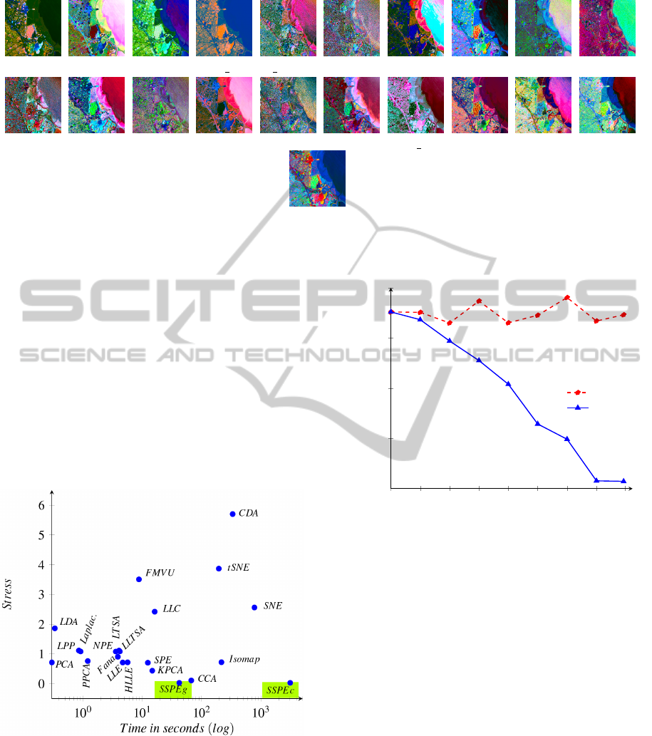
PCA CCA CDA Fact ana F MVU HLLE Isomap KPCA Laplacian LDA

LLC LLE LLTSA LPP LTSA NPE Prob PCA SPE SNE tSNE

SSPE

Figure 4: Visualization of region 1 by using 21 DR methods. According to the Table 3, the worst visualization is got by

Laplacian method, and SSPE’s visualization is the best visualization among them.

The speed is the next important item which should

be addressed. The DR idea is much faster than our

proposed method. Thus, GPU is the best way to speed

up the SDR method, that is, where the speed of exe-

cution has been increased by 74 times than when it

ran on CPU, as in the Figure 6. Thus, the speed prob-

lem that occurs in SDR is solved. Interestingly, the

consumed time by the proposed method is important

where the error is gradually lessened until it reaches

to be up to less than what can be. Figure 7 shows the

efﬁciency of the DR method (represented by SPE) is

not affected by increasing the iteration number.

Figure 6: The role of using GPU was very positive to in-

crease the speed of proposed method (SSPE) from 3107.147

seconds in CPU (which is called SSPE

) to 42.049 seconds

in GPU (which is called SSPE

). Thus, the execution speed

of SDR is acceptable when comparing that with those of

other methods.

Even though our method gave good results when

the sequences of multiple dimensionality reduction

3.3

3.6

3.9

4.2

4.51

4.81

5.11

5.4

0.2

0.4

0.6

0.8

Iteration (log)

Stress

SPE

SSPE

Figure 7: SPE and SSPE use the same number of iterations.

In SPE, there is no signiﬁcant impact on the change in SPE’s

efﬁciency through iterations, but the stress is reduced grad-

ually with SSPE.

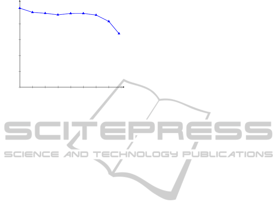
are reduced by amount equal to one, this amount can

be larger than one. However, the efﬁciency of SDR is

reduced when S is increased, as in Figure 8.

5 CONCLUSIONS

A new method called SDR has been proposed in this

paper to visualize remote sensing imagery. Theoreti-

cally, we illustrated that SDR maintains and preserves

the relations among neighbour points in low dimen-

sionality space. The results showed the accuracy of

the proposed SDR which leads to a better visualiza-

tion with minimum false colours compared to the di-

rect projection of DR method, where those results

were conﬁrmed by comparisons of our method with

20 other methods. It has been also demonstrated that

VisualizationofRemoteSensingImagerybySequentialDimensionalityReductiononGraphicsProcessingUnit

0.3

0.6

0.9

1.2

1.51

1.81

2.11

2.4

0.2

0.4

0.6

0.8

Amount o f dimensionality reduction (log)

Correlation

Figure 8: The correlation measurement value of SDR is

very high (which is equal to 0.998) when the amount of di-

mensionality reduction is equal to 1. The efﬁciency of SDR

is reduced when this reduction amount is greater than 1,

and the lowest correlation value is (0.676) when reduction

amount is equal to 223.

the speed of SDR on GPU is much faster than it is on

CPU.

ACKNOWLEDGEMENTS

It would not have been possible to write this paper

without the help and support of the Ministry of Higher

Eduction and Scientiﬁc Research in Iraq. The authors

would like to acknowledge the ﬁnancial and academic

support of the Basrah and Bangor Universities.

REFERENCES

Agraﬁotis, D. K., Xu, H., Zhu, F., Bandyopadhyay, D.,

and Liu, P. (2010). Stochastic proximity embedding:

Methods and applications. Molecular Informatics,

29:758–770.

Ameer, P. M. and Jacob, L. (2012). Localization us-

ing stochastic proximity embedding for underwater

acoustic sensor networks. In 2012 National Confer-

ence on Communications (NCC).

AVIRIS (2013). http://aviris.jpl.nasa.gov/index.html.

Bachmann, C. M., Ainsworth, T. L., and Fusina, R. A.

(2005). Exploiting manifold geometry in hyperspec-

tral imagery. IEEE transaction on geoscience and re-

mote sensing, 43:441–454.

Belkin, M. and Niyogi, P. (2002). Laplacian eigenmaps

and spectral techniques for embedding and clustering.

Advances in Neural Information Processing Systems,

14:585591.

Blum, R. S. and Liu, Z. (2006). Multi-sensor Image Fusion

and its Applications. Taylor & Francis Group.

Borg, I. and Groenen, P. J. (1997). Modern Multidimen-

sional Scaling : Theory and Applications. Springer-

Verlag, NewYork.

Bunte, K., Haase, S., Biehl, M., and Villmann, T. (2012).

Stochastic neighbor embedding (sne) for dimension

reduction and visualization using arbitrary diver-

gences. Neurocomputing, 90:23–45.

Darlington, R. B. (1999). Factor analysis. Technical report,

Cornell University,.

Demartines, P. and Hrault, J. (1997). Curvilinear compo-

nent analysis: a self-organizing neural network for

nonlinear mapping of data sets. IEEE Transactions

on Neural Networks, 8:148–154.

Donoho, D. L. and Grimes, C. (2005). Hessian eigenmaps:

New locally linear embedding techniques for high-

dimensional data. In The National Academy of Sci-

ences, 102(21):74267431.

Duda, R. O., Hart, P. E., and Stork, D. G. (2001). Pattern

Classiﬁcation. Wiley Interscience Inc.

He, X., Cai, D., Yan, S., and Zhang, H.-J. (2005). Neigh-

borhood preserving embedding. In Tenth IEEE Inter-

national Conference on Computer Vision (ICCV) (Vol-

ume:2 ).

Jolliffe, I. (2002). Principal Component Analysis. Springer

Verlag, New York, Inc.

Kaski, S. and Peltonen, J. (2011). Dimensionality reduction

for data visualization. IEEE signal processing maga-

zine, 28:100–104.

Lawrence, J., Arietta, S., Kazhdan, M., Lepage, D., and

OHagan, C. (2011). A user-assisted approach to

visualizing multidimensional images. IEEE Trans-

action on Visualization and Computer Graphics,

17(10):1487–1498.

Lee, J. A., Lendasse, A., and Verleysen, M. (2004). Non-

linear projection with curvilinear distances: Isomap

versus curvilinear distance analysis. Neurocomputing,

57:49–76.

Lespinats, S. and Aupetit, M. (2011). Checkviz: Sanity

check and topological clues for linear and non-linear

mappings. Comput. Graph. Forum, 30:113–125.

Maaten, L. V. D. and Hinton, G. (2008). Visualizing data us-

ing t-sne. Machine Learning Research, 9:2579–2605.

Maaten, L. V. D., Postma, E., and Herik, H. V. D. (2009).

Dimensionality reduction: A comparative review. Ma-

chine Learning Research, 10:1–41.

Mignotte, M. (2012). A bicriteria-optimization-approach-

based dimensionality-reduction model for the color

display of hyperspectral images. IEEE Transactions

on Geoscience and Remote Sensing, 50:501–513.

Mokbel, B., Lueks, W., Gisbrecht, A., and Hammera, B.

(2013). Visualizing the quality of dimensionality re-

duction. Neuocomputing, 112:109–123.

Peltonen, J. (2009). Visualization by linear projections as

information retrieval. Advances in Self-Organizing

Maps Lecture Notes in Computer Scienc, 5629:237–

245.

Roweis, S. T. and Saul, L. K. (2000). Nonlinear dimension-

ality reduction by locally linear embedding. science,

290:2323–2326.

Sanders, J. and Kandrot, E. (2011). CUDA by example.

Addison-Wesley Professional.

IVAPP2014-InternationalConferenceonInformationVisualizationTheoryandApplications

Shawe-Taylor, J. and Cristianini, N. (2004). Kernel methods

for pattern analysis. Cambridge University Press.

Shi, J. and Malik, J. (2000). Normalized cuts and image

segmentation. IEEE Transaction on Pattern Analysis

and Machine Intelligence, 22:888–905.

Smith, R. B. (2012). Introduction to Hyperspectral Imag-

ing. MicroImages, Inc.

Steyvers, M. (2002). Multidimensional scaling. Encyclope-

dia of Cognitive Science.

Tenenbaum, J. B., de Silva, V., and Langford, J. C. (2000).

A global geometric framework for nonlinear dimen-

sionality reduction. Science 290, 5500:2319–2323.

Tipping, M. E. and Bishop, C. M. (1999). Mixtures of prob-

abilistic principal component analyzers. Neural Com-

putation, 61:611.

Tyo, J. S., Konsolakis, A., Diersen, D. I., and Olsen, R. C.

(2003). Principal-components-based display strategy

for spectral imagery. IEEE transactions on geoscience

and remote sensing, 41:708718.

Venna, J., Peltonen, J., Nybo, K., Aidos, H., and Kaski, S.

(2010). Information retrieval perspective to nonlin-

ear dimensionality reduction for data visualization. J.

Mach. Learn. Res, 11:451–490.

Weinberger, K. Q. and Saul, L. K. (2006). An introduction

to nonlinear dimensionality reduction by maximum

variance unfolding. In Proceedings of the National

Conference on Artiﬁcial Intelligence, Boston, MA.

Zhang, T., Yang, J., Zhao, D., and Ge, X. (2007). Linear

local tangent space alignment and application to face

recognition. Neurocomputing, 70:1547–1553.

Zhang, Z. and Zha, H. (2004). Principal manifolds and

nonlinear dimensionality reduction via local tangent

space alignment. SIAM Journal of Scientiﬁc Comput-

ing, 26:313–338.

Zhi, R. and Ruan, Q. (2008). Fractional supervised orthog-

onal local linear projection. In CISP ’08. Congress on

(Volume:2 ) Image and Signal Processing.

VisualizationofRemoteSensingImagerybySequentialDimensionalityReductiononGraphicsProcessingUnit