
Unsupervised Segmentation of Hyperspectral Images based on
Dominant Edges
Sangwook Lee, Sanghun Lee and Chulhee Lee
Department of Electrical and Electronic Engineering, Yonsei University, 50, Yonsei-ro, Seodaemun-gu, Seoul, Korea
Keywords: Segmentation, Hyperspectral Images, PCA, Dominant Edges.
Abstract: In this paper, we propose a new unsupervised segmentation method for hyperspectral images based on
dominant edge information. In the proposed algorithm, we first apply the principal component analysis and
select the dominant eigenimages. Then edge operators and the histogram equalizer are applied to the
selected eigenimages, which produces edge images. By combining these edge images, we obtain a binary
edge image. Morphological operations are then applied to these binary edge image to remove erroneous
edges. Experimental results show that the proposed algorithm produced satisfactory results without any user
input.
1 INTRODUCTION
Hyperspectral images have been successfully used in
many remote sensing applications, which include
classifications (Guo, 2006), target detections and
environment monitoring (Wang, 2003). In
automated processing of remotely sensed images,
segmentation is an important first step. With good
unsupervised segmentation algorithms, it is
generally possible to enhance the performance of
many operations (Cao, 2007).
In general, the goal of segmentation is to divide
images into their constituent regions. However, in
natural scenes, images often contain roads, tree,
buildings, fields, ponds, etc. Furthermore, there may
be no clear boundaries between the different regions.
Consequently, segmentation can be a complex and
difficult operation. The segmentation process can be
either unsupervised or supervised. Supervised
segmentation methods require training data and the
application areas of these methods are rather limited.
However, unsupervised segmentation methods,
which do not require any advanced information,
have larger application areas.
Among the various unsupervised segmentation
methods, the clustering technique has been most
widely used. This technique includes the k-means
method and the ISODATA method (Roberts 1997,
Meyer 2003). However, it is difficult to apply these
methods to hyperspectral images due to prohibitive
computational costs and the difficulty of selecting
initial points. Furthermore, performance can be
rather limited. Efforts have been made to develop
segmentation algorithms for hyperspectral images.
The morphological method has been proposed to
segment hyperspectral images, which use pixel
similarities (Pesaresi 2001). A MRF (Markov
Random Field) model segmentation method has
been proposed, which was based on capturing the
intrinsic characteristics of tonal and textural regions
(Sarkar 2002). In order to segment hyperspectral
images accurately, a number of techniques have
been employed, such as mutual information, phase
correlation and convex cone analysis (Guo 2006,
Erturk 2006, Ifrarraguerri 1999). Statistical
segmentation methods have also used a Gaussian
mixture model and stochastic estimation
maximization (Acito 2000, Masson 1993). Recently,
segmentation based on watershed transformation has
been proposed (Tarabalka 2010) and Tarabalka et al.
proposed a segmentation and classification method
using automatically selected markers (Tarabalka
2010).
In this paper, we propose a new unsupervised
segmentation method, which is based on edge
information and utilizes a post-processing technique
to improve segmentation results.
588
Lee S., Lee S. and Lee C..
Unsupervised Segmentation of Hyperspectral Images based on Dominant Edges.
DOI: 10.5220/0004739705880592
In Proceedings of the 9th International Conference on Computer Vision Theory and Applications (VISAPP-2014), pages 588-592
ISBN: 978-989-758-003-1
Copyright
c
2014 SCITEPRESS (Science and Technology Publications, Lda.)
2 SEGMENTATION USING EDGE
FUSION AND REGION
GROWING
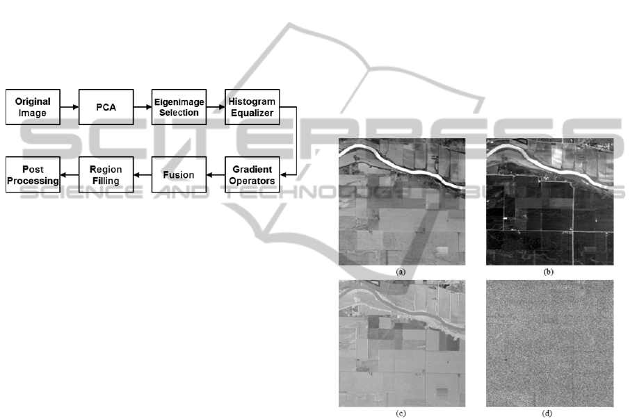
Fig. 1 shows a block diagram of the proposed
method. First, we apply the principal component
analysis using the method described in (Lim S, 2001)
and select the dominant eigenimages. Then edge
operators are applied to find the edge pixels. This
procedure is repeated for each of the retained
dominant eigenimages and the edge images are then
combined to produce a reference edge image.
Finally, we apply morphological operations and
post-processing to improve the segmentation results.
Figure 1: Block diagram of the proposed method.
2.1 Gradient Operators
Fig. 2 shows some eigenimages. The first three
eigenimages corresponding to the largest
eigenvalues retained about 99% of the total energy,
which is the squared sum of all the pixels. In the
proposed method, we applied an edge detection
algorithm and histogram equalizer to the three
eigenimages after performance evaluation on the
number of eigenimages. To acquire the edges of
eigenimages, we applied gradient operators as
follows:
),(*),(),(
),(),(),(
nmRbnm
i
EGnm
i
R
nmSbnm
i
EGnm
i
S
(1)
where
),( nmEG
i
is the i-th eigenimage and
),( nmSb
and
),( nmRb
are the Sobel operator and the
Robinson operator.
),( nmS
i
and ),( nmR
i
are the i-
th the Sobel and the Robinson edge image. Mainly
horizontal and vertical edge components are
produced by the Sobel filter and diagonal edge
components are acquired by the Robison filter. We
applied this procedure to the selected eigenimages
and obtained the corresponding edge images.
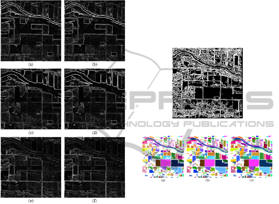
Therefore, 6 edge images were produced. Fig. 3
shows the edge images.
Then we applied the threshold operation to the
edge images and obtained binary edge images. The
threshold value was computed from the mean and
variance of the edge image as follows:
kThreshold
(2)
where
and
represent the mean and standard
deviation values, which were calculated from the
edge images. In (2),
k
is a coefficient, which we set
to 0.35, which was chosen empirically after testing
different coefficients. To combine the edge images,
we computed the union and intersection edge images
and the reference binary edge image are produced as
follows:
),()...,(),(),(
21
nmEInmEInmEInmE
n
(3)
where
),( nmEI
j
is the j-th edge image and ),( nmE
is the reference binary edge image (Fig. 4).
Figure 2: The eigenimages (a) the 1st eigenimage, (b) the
3rd eigenimage, (c) the 5th eigenimage and (d) the 7th
eigenimage.
2.2 Morphological Operations and Post
Processing
We can view the edges of the reference binary edge
images as boundaries between regions. The
reference binary edge image contains a number of
regions (connected components), which can be
found using a connected component labeling
algorithm. However, some of the connected
components may be small. We select the connected
components whose sizes are larger than a threshold
value. In this paper, we empirically set the threshold
value as 22. Connected components may contain
UnsupervisedSegmentationofHyperspectralImagesbasedonDominantEdges
589
many small holes. To eliminate these holes, we
apply a region filling method. Fig. 5(b) shows the
output image after the region filling method was
applied.
Figure 3: The edge images of the selected eigenimages (a)
the Sobel edge image of the 1
st
eigenimage, (b) the Sobel
edge image of the 2
nd
eigenimage, (c) the Sobel edge
image of the 3
rd
eigenimage, (d) the Robinson edge image
of the 1
st
eigenimage, (e) the Robinson edge image of the
2
nd
eigenimage and (f) the Robinson edge image of the 3
rd
eigenimage.
Pixels at boundaries may generally be unclassified
even after performing the region filling procedure,
even if they belong to a region. In order to assign
these kinds of pixels to one of the identified regions,
we compute the mean vector and covariance matrix
of each region (connected component). Assuming
that each region could be approximated by a normal
distribution, for each unclassified pixel within 5
pixels from the boundary pixels, we compute the
following chi-square distribution:
)()()(
1
ii
t
ii
mxmxxy
(4)
where
x
represents an unclassified pixel,
i
m
represents the mean vector of the i-th region and
i
represents the covariance matrix of the i-th region. If
)(xy
i
is smaller than the threshold value and
)()( xyxy
ji
, we assign the pixel to the i-th region
where j refers to all neighbour connected
components other than the i-th region. Fig. 5(c)
shows the final segmented image after post-
processing.
Figure 4: Reference binary edge image.
Figure 5: (a) An image before region growing, (b) an
image after region fills, and (c) the segmented image after
post processing.
3 EXPERIMENTAL RESULTS
We evaluated the performance of the proposed
algorithm using the AVIRIS (Airborne
Visible/Infrared Imaging Spectrometer) over some
agricultural areas. There are 220spectral bands in the
0.4 to 2.4 µm regions. This data set contains 2166
scan lines with 614 pixels in each scan line. From
the data set, we selected a sub-region of 613 613
pixels.
The proposed method produced a good
segmentation result although it is completely
automated. Most fields were correctly identified
with clear boundaries. Next, the proposed algorithm
was compared with the k-means algorithm. In order
to apply the k-means method, the spectral bands of
the original hyperspectral image were reduced by
averaging the four adjacent spectral bands. The
VISAPP2014-InternationalConferenceonComputerVisionTheoryandApplications
590
averaging procedure would eliminate the noise
factors of the spectral bands. The segmentation
results of the two methods are shown in Fig. 6. The
proposed method produced a much better result than
the k-means method. The proposed method was also
faster than the k-means method by 4.29 times in
terms of processing time.
Table 1: Information of reconstruction images when using
the proposed algorithm.
Group Field Area Correct
(%)
Incorrect
(%)
No.
detect
(%)
1 Tree 168 0.0% 0.0 100.0
2 Corn1 578 99.7 0.0 0.3
3 Water 80 100.0 0.0 0.0
4 Pasture1 360 99.2 0.0 0.8
5 Corn2 360 14.2 0.0 85.8
6 Corn3 416 62.0 0.0 38.0
7 Pasture2 333 95.5 0.0 4.5
8 Corn4 792 97.3 0.0 2.7
9 Wheat 774 99.7 0.0 0.3
10 Soy1 792 96.8 0.0 3.2
11 Corn5 684 82.3 0.0 17.7
12 Corn6 1107 88.6 0.0 11.4
13 Soy2 1400 99.5 0.0 0.5
14 Corn7 1800 99.7 0.0 0.3
15 Corn8 540 81.5 0.6 18.0
16 Soy3 450 96.7 0.0 3.3
17 Corn9 480 97.9 0.0 2.1
18 Soy4 324 50.3 0.0 49.7
19 Soy5 1482 99.8 0.0 0.2
20 Soy6 594 99.8 0.0 0.2
21 Soy7 952 43.9 10.2 45.9
Total - 14466 81.1638 0.5116 18.3245
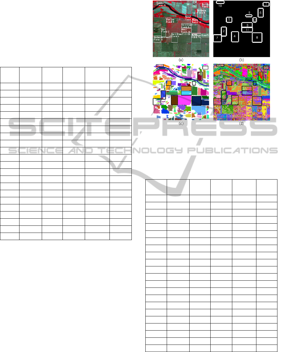
In order to provide quantitative analyses, we
selected 12 classes from the AVIRIS data, as shown
in Fig. 6(a). Table 1 shows the class description. It
also shows the percentile of correctly classified
pixels and incorrectly classified pixels. The
proposed method produced a much better result than
the k-means method (Table 2). It is noted that the
proposed method may produce a number of
unclassified pixels.
4 CONCLUSIONS
In this paper, we have proposed a completely
automated segmentation method. The key idea of the
proposed method is to use the edge information of
the dominant eigenimages. Although the proposed
method is unsupervised and does not require any
Figure 6: Performance comparisons: (a) the truth map, (b)
number of regions (c) the result of the proposed
algorithm, and (d) the result of the k-means algorithm.
Table 2: Information of reconstruction images when using
the k-means algorithm.
Group Field Area
Correct
(%)
Incorrect
(%)
No.
detect
(%)
1 Tree 168 21.4 78.6 0
2 Corn1 578 41.7 58.3 0
3 Water 80 100 0 0
4 Pasture1 360 66.9 33.1 0
5 Corn2 360 24.2 75.8 0
6 Corn3 416 48.0 51.92 0
7 Pasture2 333 61 39 0
8 Corn4 792 42.1 57.9 0
9 Wheat 774 56.7 43.3 0
10 Soy1 792 39.8 60.2 0
11 Corn5 684 37.7 62.3 0
12 Corn6 1107 44.8 55.2 0
13 Soy2 1400 62.4 37.6 0
14 Corn7 1800 55 45 0
15 Corn8 540 41.3 58.7 0
16 Soy3 450 52.7 47.3 0
17 Corn9 480 78.6 21.4 0
18 Soy4 324 66.8 33.2 0
19 Soy5 1482 41.1 58.9 0
20 Soy6 594 40.6 59.4 0
21 Soy7 952 35 65 0
Total - 14466 50.5 49.5 0
user intervention, it can provide fairly good
segmentation results. The proposed algorithm is
relatively simple and easy to implement, and it
UnsupervisedSegmentationofHyperspectralImagesbasedonDominantEdges
591

compares favourably with existing unsupervised
methods.
REFERENCES
Acito N, Corsini G and Diani M 2000. An unsupervised
algorithm for hyperspectral image segmentation based
on the Gaussian mixture model. in Proc, IGARSS, pp.
3745-3747.
Cao F, Hong W, Wu Y and Pottier E 2007. An
Unsupervised Segmentation With an Adaptive
Number of Clusters Using the SPAN/H/α/A Space and
the Complex Wishart Clustering for Fully Polarimetric
SAR Data Analysis. IEEE Trans., Geosci. Remote
Sens., vol. 45, no.11, pp. 3454-3467.
Erturk A and Erturk S 2006 . Unsupervised Segmentation
of Hyperspectral Images Using Modified Phase
Correlation. IEEE Geosci. Remote Sens. Lett., vol. 3,
no. 4, pp. 527-531.
Guo B. Gunn S. R. and Damper R. I. 2006. Band Selection
for Hyperspectral Image Classification Using Mutual
Information. IEEE Geosci. Remote Sens. Lett., vol. 3,
no. 4, pp. 522-526.
Ifrarraguerri A and Chang C. I. 1999. Multispectral and
hyperspectral image analysis with convex cones. IEEE
Trans., Geosci. Remote Sens., vol. 37, no. 2, pp. 756 –
770.
Lim S, Sohn K and Lee C 2001. Principal Component
Analysis for Compression of Hyperspectral Images.
Proc. IEEE IGARSS, vol. 1, pp. 97-99.
Masson P and Pieczynski W 1993. SEM algorithm and
unsupervised statistical segmentation of satellite
images. IEEE Trans., Geosci, and Remote Sens., vol.
31, no. 3, pp. 618– 633.
Meyer A, Paglieroni D and Astaneh C 2003. K-means re-
clustering: Algorithmic options with quantifiable
performance comparisons. Proceedings of the SPIE,
Volume 5001, pp. 84-92.
Pesaresi M and Benediktsson A 2001. A New Approach
for the Morphological Segmentation of High-
Resolution Satellite Imagery. IEEE Trans., Geosci.
Remote Sens., vol. 39, no. 2, pp. 309-320.
Robert AS 1997. Remote sensing: models and methods for
image processing. Academic Press, 2nd edit., pp. 389-
447.
Sarkar A, Biswas M. K. and Kartikeyan B 2002. A MRF
Model-Based segmentation Approach to classification
for Multispectral imagery. IEEE Trans., Geosci.
Remote Sens., vol. 40, no. 5, pp. 1102-1113.
Tarabalka Y, Chanussot J, and Benediktsson J. A. 2010.
Segmentation and Classification of Hyperspectral
Images Using Minimum Spanning Forest Grown From
Automatically Selected Markers. IEEE Trans.
Systems, Man, and Cybernetics—PART B:
Cybernetics, vol. 40, no. 5, pp. 1267 – 1279.
Tarabalka Y, Chanussota J, and Benediktsson JA 2010.
Segmentation and classification of hyperspectral
images using watershed transformation. Pattern
Recognition, vol. 43, Iss. 7, pp. 2367–2379.
Wang S, Yan F, Zhu L, Wang L and Jiao Y 2003. Water
quality monitoring using hyperspectral remote sensing
data in Taihu Lake China. Proc., IGARSS, pp. 4553-
4556.
VISAPP2014-InternationalConferenceonComputerVisionTheoryandApplications
592
