Assisting Navigation in Homogenous Fog

Mihai Negru and Sergiu Nedevschi

Computer Science Department, Technical University of Cluj-Napoca, Cluj-Napoca, Romania

Keywords: Driving Assistance Systems, Fog Detection, Visibility Distance Estimation, Speed Recommendation.

Abstract: An important cause of road accidents is the reduced visibility due to the presence of fog or haze. For this

reason, there is a fundamental need for Advanced Driving Assistance Systems (ADAS) based on efficient

real time algorithms able to detect the presence of fog, estimate the fog’s density, determine the visibility

distance and inform the driver about the maximum speed that the vehicle should be traveling. Our solution

is an improvement over existing methods of detecting fog due to the temporal integration of the horizon line

and inflection point in the image. Our method performs in real time; approximately 50 frames per second. It

is based on a single in-vehicle camera and is able to detect day time fog in real time in a wide range of

scenarios, including urban scenarios.

1 INTRODUCTION

During the last decade a special attention was given

to advanced driving assistance systems. Nowadays

vehicles are equipped with active safety systems, in

order to reduce the number of traffic accidents. Thus

an important aspect, for avoiding accidents and

reducing the risk of accident, while driving, is the

ability of an advanced driving assistance system to

anticipate such risks and to notify the driver of the

hazardous situations. The National Highway Traffic

Safety Administration (NHTSA) states that the top

six most common causes of automobile crashes are:

distracted drivers, speeding, aggressive driving,

drunk driving, driver fatigue and weather

phenomena. In the case of driver inattention 80% of

accidents happen due to 3 seconds of distraction.

Even though there is a significant improvement in

road infrastructure the number of accidents caused

by extreme weather conditions is higher every year.

Among these conditions fog is considered to be the

most dangerous one because the visibility distance

decreases exponentially as fog density increases.

When the weather is affected by fog, drivers tend to

overestimate the visibility distances and drive with

excessive speed (Hautiere et al., 2006). For this

reason we developed a system for assisting the

driver in foggy situations. Our system is capable of

detecting the presence of fog in images, measuring

the visibility distance in such situations and

informing the driver about the maximum speed that

they should travel on the given road segment. An

important improvement of our method consists in

the fact that the horizon line and the inflection point

are detected frame-by-frame and then time filtered,

resulting in a very stable and reliable solution for fog

detection. Our solution performs in real time

(approximately 50 frames per second). It can be

ported easily on a modern smartphone or tablet,

making it an inexpensive and very accessible ADAS

solution. In addition the detection results could be

transmitted to a regional traffic information system

that gathers and distributes weather information in

real time.

2 RELATED WORK

Fog detection systems were studied in the past years

with the aim of detecting the presence of fog and

removing the fog effects from images. Pomerleau

(Pomerleau, 1997) estimates visibility in fog

conditions by means of contrast attenuation at road

markings in front of the vehicle. This approach

requires the presence and detection of road

markings. Another approach consists in the

combination of an in-vehicle camera and radar (Mori

et al., 2006). Based on Koschmieder’s law they

classify the fog density according to a visibility

feature of a preceding vehicle.

In (Bronte et al., 2009) a method for fog

detection based on the computation of the vanishing

619

Negru M. and Nedevschi S..

Assisting Navigation in Homogenous Fog.

DOI: 10.5220/0004740006190626

In Proceedings of the 9th International Conference on Computer Vision Theory and Applications (VISAPP-2014), pages 619-626

ISBN: 978-989-758-004-8

 2014 SCITEPRESS (Science and Technology Publications, Lda.)

point is presented. The road lines are taken as

reference lines in order to compute the vanishing

point. After the vanishing point is found a

segmentation of the road and sky is performed. This

method is able to classify fog based on its density.

Object detection on foggy images is presented in

(Dong et al., 2011). The method uses a fixed camera

and performs object detection based on the

subtraction of the observed dense map and a

background depth map. The drawback of this

method is that it cannot be used in real traffic scenes,

where the background scenario is continuously

changing.

In (Pavlic et al., 2012) an approach based on

image descriptors and classification is used in order

to detect fog conditions. The image descriptors used

are Gabor Filters at different frequencies, scales and

orientations. The visibility distance estimation in fog

conditions is presented in (Hautiere et al., 2006).

Their algorithm is based on Koschmieder’s law and

is able to detect the visibility distance in day time

traffic scenarios. In order to assess if fog is present

in images they use a region growing procedure for

detecting the inflection point in the image. Knowing

the position of the inflection point and the horizon

line position (that is computed offline) they are able

to compute the visibility distance in the image.

Because accidents that happen during fog

conditions result in a high number of casualties,

there is a growing concern in providing assistance to

the drivers. One such approach was implemented by

the California Department of Transportation

(Berman et al., 2009). They have developed a fog

detection and warning system based on an array of

sensors able to detect fog. These sensors are

deployed every half mile on both direction of a

freeway. In addition this system is able to provide

drivers with information about the fog density and

the maximum speed that they should travel. The

information is displayed on Changeable Message

Signs. Although it is a very expensive system the

fact that the drivers are informed about the weather

conditions and speed limits reduced drastically the

number of accidents on this highway. Our intention

is to develop a more cost effective approach to the

problem of fog detection and to inform the driver

about the maximum speed on the given road

segment.

3 MODELING THE EFFECTS OF

FOG ON VISION

3.1 Koschmieder’s Law

In 1924, Koschmieder (Middleton, 1952) studied the

attenuation of luminance through the atmosphere

and proposed a relationship between the attenuation

of an object’s luminance L at distance d and the

luminance L

close to the object:

(1 )

kd kd

LLe L e







(1)

∞

is the atmospheric luminance and k is the

extinction coefficient. This equation states that the

luminance of an object seen through fog is

attenuated with an exponential factor e

-kd

; the

atmospheric veil obtained from daylight scattered by

fog between the object and the observer is expressed

by L

∞

(1-e

-kd

). By re-writing this equation and

dividing by L

∞

we obtain Duntley’s attenuation law

(Hautiere et al., 2006) that states that an object

having the contrast C

with the background is

perceived at distance d with contrast C:

()

kd kd

CeCe









(2)

This law can be applied only in day light uniform

illumination conditions. From this expression the

meteorological visibility distance is derived (d

vis

“the greatest distance at which a black object, having

contrast (C

=1), of a suitable dimension can be seen

in the sky on the horizon”. In order for an object to

be barely visible, the International Commission on

Illumination has adopted a threshold for the contrast,

i.e. 5%. It results that:

log(0.05)

vis

 

(3)

When dealing with images, the response function

of a camera can be applied to the Koschmieder’s

equation in order to model the mapping from scene

luminance to image intensity. Thus, the intensity

perceived in the image is the result of a function (f)

applied to equation (1):







kd kd

IfL Re A e







(4)

∞

is the sky intensity and R is the intrinsic pixel

intensity.

VISAPP2014-InternationalConferenceonComputerVisionTheoryandApplications

620

3.2 Modelling the Camera in the

Vehicle Environment

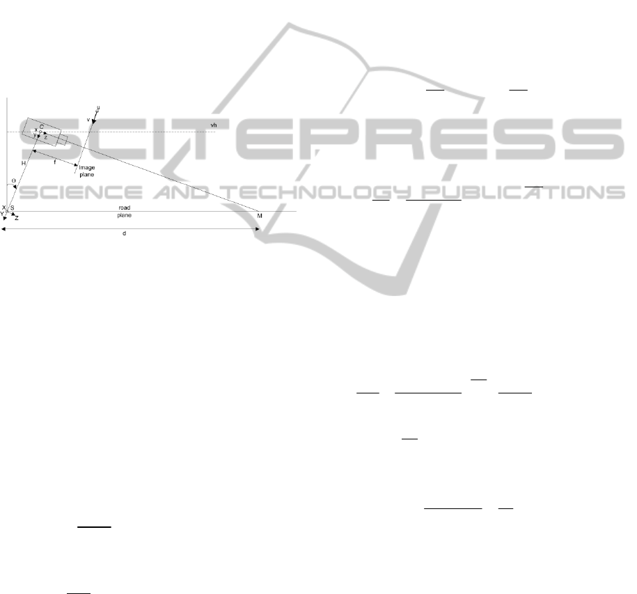
Figure 1 presents a typical camera system mounted

inside a vehicle. The position of a pixel in the image

plane is given by its (u, v) coordinates, the position

of the optical center C is given by (u0, v0) and f

represents the focal length of the camera. Nowadays

cameras usually have square pixels, so the horizontal

pixel size tpu is equal to the vertical pixel size tpv,



t



t



) thus we can introduce a new

constant denoted by αf/t



in order to express the

value of the focal length in pixels. The camera is

mounted at height H relative to the S(X, Y, Z)

coordinate system and θ represents the pitch angle.

Figure 1: The camera model in the vehicle environment.

From Figure 1 one can observe that the

horizontal line passing through the optical center

makes an angle θ with the z axis. Therefore it can be

expressed as:

tan







(5)

In the case of a single camera, the flat world

hypothesis can be used to estimate the distance to

each line in the image (Negru and Nedevschi, 2013).

This hypothesis is used in the case of road scene

images, since a large part of an image is formed by

the road surface, which can be assumed to be planar.

So, the distance d of an image line v, can be

expressed by the following equation:

if v v





















(6)

Where 



 

and v

represents the horizon line in

the image. The value of d from equation (6) will be

used in order to assess the visibility distance in fog

conditions.

4 METHOD DESCRIPTION

4.1 Estimation of the Visibility

Distance

In order to estimate the visibility distance we must

first examine the mathematical properties of the

Koschmieder’s law, presented in the previous

section. For estimating the extinction coefficient k

we must investigate the existence of an inflection

point in the image that will provide the basis for our

solution. By expressing d as in equation (6) and by

performing a change of variable, equation (4)

becomes:

(1 )

vv vv

IRe A e









(7)

If we take the derivative of I with respect to v,

taking into account that the camera response is a

linear function, one obtains:



()

dI k











(8)

We know that objects tend to get obscured more

quickly when fog density increases. Moreover, the

maximum derivative decreases significantly and

deviates more substantially from the horizon line. So

the inflection point in the image can be found where

the derivative has a maximum value. By computing

again the derivative of I with respect to v, we get the

following equation:



()

kRAdI k

dv v v





















(9)

Equation









0 has two possible solutions. We

search for a positive solution of k, so k=0 is not

acceptable. Thus the solution obtained is:

2( )







(10)

represents the position of the inflection point

in the image and d

represents its distance to the

camera.

If we are able to compute the position of the

inflection point and of the horizon line we can

compute the extinction coefficient from

Koschmieder’s law. If v

is greater than v

fog will

be detected in the image, otherwise we conclude that

there is no fog in the scene. From equations (3) and

(10) we can estimate the visibility distance in the

image:

AssistingNavigationinHomogenousFog

621

2( )

vis







(11)

Using this visibility distance and taking into

account the braking distances at various speeds, we

can infer the fog density and the maximum safe

driving speed of the vehicle should.

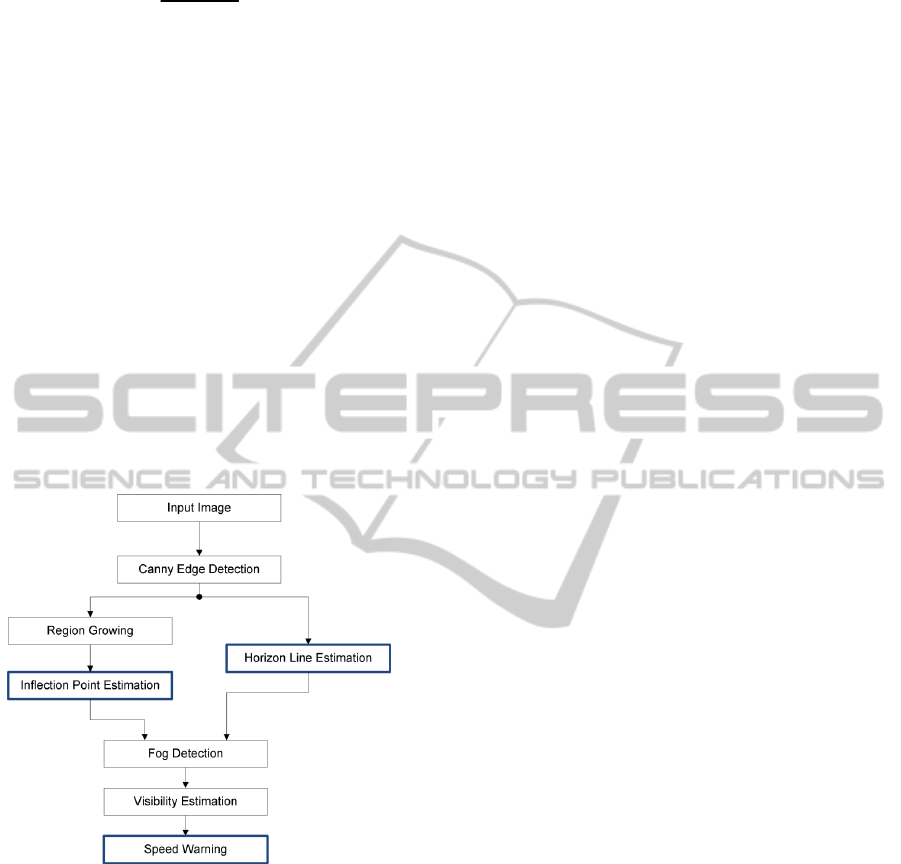
4.2 Algorithm Overview

The architecture of our framework is presented in

Figure 2. The main contributions of our work are in

the blue highlighted areas. Our method uses grey

scale images as input and is able to provide

information about the presence of fog in the image

and to estimate the maximum speed on the given

road segment. First we apply a Canny-Deriche edge

detector on the input image. Then we estimate the

horizon line and the inflection point in order to

assess whether fog is present in the image. If fog is

present in the image, then we perform visibility

estimation and speed warning recommendation.

Figure 2: System Architecture.

4.2.1 Horizon Line Estimation

Several methods can be employed for computing the

horizon line in the image. The first one relies on

using a simple calibration procedure to compute the

pitch angle of the camera (Hautiere et al., 2006). An

alternative, our choice, is to estimate the horizon line

based on the image features. This will ensure a

better result for the horizon line estimation in

different traffic situations.

The horizon line in the image will be detected by

finding the vanishing point of the painted quasi-

linear and parallel (in 3D) road features such as lane

markings. In (Bronte et al., 2009) only the two

longest lines are considered for finding the vanishing

point. We prefer a more statistical approach that uses

more lines and was previously used to find the

vanishing point of the 3D parallel lines from

pedestrian crossings (Se, 2000). The main steps for

the detection of the vanishing point are:

1. Select a set of relevant lines in the half lower

part of the image (road area). The Hough

accumulator was built from the edge points in the

interest area. The highest m peaks were selected

from the accumulator, and those that were having at

least n votes were validated as the relevant lines.

2. A RANdom SAmple Consensus (RANSAC)

approach is applied to find the largest subset of

relevant lines that pass through the same image

point. A number of K (=48 for a success probability

p=0.99 and percentage of good lines w=0.3) random

samples of two relevant lines are selected. For each

sample the intersection P of the two lines is

computed and consensus set is determined as the

subset of relevant lines that pass through P (within a

small circle around P). The sample having the

largest consensus set is selected.

3. The intersection points of each distinct pair of

lines from the largest consensus set are computed.

Finally, the vanishing point is computed as the

center of mass of the intersection points.

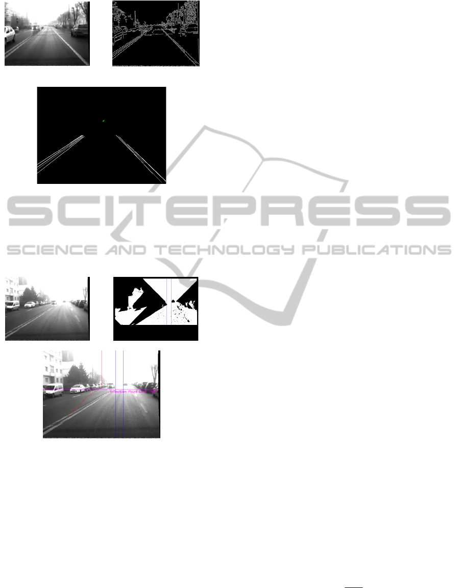
Figure 3 presents the results of applying the

horizon line detection process. The bottom image

presents only the detected Hough lines that form the

consensus set and their intersection points in green

colour.

Using this RANSAC approach for computing the

vanishing point provides an additional benefit. The

consensus score of the best pair of lines can be used

in a temporal scheme to deal with scenes that lack

painted lane markings: the vanishing point with the

highest consensus score is selected from the last N

frames. N can be chosen large enough to ensure the

car has travelled along multiple road segments. This

temporal integration makes the horizon line

detection algorithm more stable.

4.2.2 Region Growing

The region growing process follows the guidelines

presented in (Hautiere et al., 2006). The objective is

to find a region within the image that displays

minimal row to row gradient variation.

Starting from a seed point only the three pixels

above the current pixel are added to the region if

they satisfy the following constraints: the pixel does

VISAPP2014-InternationalConferenceonComputerVisionTheoryandApplications

622

Original Image Edge Image

Hough Image with the intersection points of the consensus

lines

Figure 3: Horizon Line estimation algorithm based on

Random Sample Consensus.

not belong to the region, it is not an edge point

and presents a similarity with the seed and the pixel

located below.

Original Image

Region Growing

Inflection Point Line Result

Figure 4: Region Growing and Inflection Point

Estimation.

4.2.3 Inflection Point Estimation

In order to compute the inflection point v

we must

first find the maximum band that crosses the region

from top to bottom (Hautiere et al., 2006). If we

cannot find such a band, then we can assume that

there is no fog in the image. Next we compute the

median value for each line of this band and we

smooth these values such that the obtained function

is strictly decreasing. We extract the local maxima

of the derivative of this function and compute the

values for k, R and A

∞

for these maxima. The point

that minimizes the square error between the model

and the measured curve is considered to be the

global inflection point v

of the image. Figure 4

illustrates the results for detecting the inflection

point line. The region growing result is displayed in

the top right image. The vertical band is presented

with blue and the smoothed median values in the

inflection point band are displayed with orange in

the bottom image. Finally, the inflection point line is

displayed in pink. In order to increase the robustness

of the inflection point computation, a temporal

scheme similar to the one for horizon line detection

is employed.

4.2.4 Fog Detection and Visibility Distance

Estimation

Once the horizon line v

and inflection point v

are computed, we can detect the presence of fog in

the image and we can estimate the visibility distance

vis

from equation (11). If the position of the

inflection point line is greater than the vertical

position of the horizon line we are able to detect fog

in the image. Based on the visibility distance

estimation we are able to classify fog into five

different categories presented in Table 1.

4.2.5 Speed Warning Recommendation

Many accidents that happen during fog conditions

are caused by excessive driving. For this reason a lot

of efforts have been made so that advanced driving

assistance systems will be able to provide good

maximum speeds for driving. A method for

determining variable speed limits taking into

account the geometry of the road, sight distance,

tyre-road friction and vehicle characteristics is

presented in (Jimenez et al., 2008). They construct

an Intelligent Speed Adaptation (ISA) system based

on a very detailed digital map. Although a lot of

information is implemented in the ISA, the system is

expensive and hard to retrofit on older vehicles. In

order to avoid any accidents in fog conditions we

consider that a “zero risk” approach would be more

cautious (Gallen et al., 2010). Thus we consider the

total stopping distance to be equal to the distance

travelled during the reaction time and the breaking

distance. So, for providing the driver with a good

recommendation of safe driving speed we consider

that the visibility distance d

vis

computed by our

method is given by the following equation

vis t r

dRv



(12)

The first term of equation (12) represents the

AssistingNavigationinHomogenousFog

623

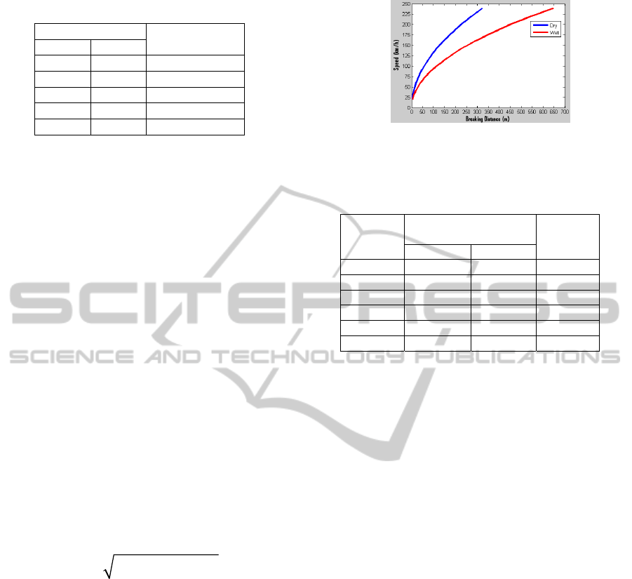
Table 1: Fog Categories.

Visibility distance

Fog

Category

Min Max

1000 m ∞ m No Fog

300 m 1000 m Low Fog

100 m 300 m Moderate Fog

50 m 100 m Dense Fog

0 m 50 m Very Dense Fog

distance travelled during the safety time margin

(including the reaction time of the driver), and the

second term is the braking distance. This is a generic

case formula and does not take into account the mass

of the vehicle and the performance of the vehicle’s

breaking and tire system.

 R

is a time interval that includes the reaction

time of the driver and several seconds before a

possible accident may occur. Because we are

aiming to obtain a cost effective solution for

warning drivers about the speed that they should

travel during fog conditions and because we do

not take into account the geometry of the road

since we do not use an augmented digital map, we

have considered this interval to be equal to 5

seconds. This covers the interval of distracted

drivers’ inattention for most of the dangerous

events that might occur during fog conditions.

 g is the gravitational acceleration, 9.8 m/s

 f is the friction coefficient. For wet asphalt

we use a coefficient equal to 0.35.

 v

denotes the recommended driving speed.

By solving equation (12) we obtain the following

positive solution for v

222

rt tvis

vgfRgfRgfd  

(13)

Figure 5 represents a plot of the braking

distances on wet and dry asphalt according to the

speed of traveling. The friction coefficient for dry

asphalt was set to 0.7 and for wet asphalt to 0.35

(EnginneringToolbox).

Table 2 presents some maximum recommended

speeds according to the fog density and the visibility

distance measured by our algorithm. In addition we

show the braking distances on wet asphalt.

According to our model of computing the

recommended speed, the driver has enough time in

order to react and to break the vehicle in case of an

emergency or hazardous event.

Figure 5: Braking distance on dry and wet asphalt. These

values were computed with the following friction

coefficients: 0.7 for dry asphalt and 0.35 for wet asphalt.

Table 2: Speed Recommendations under Fog Conditions.

Visibility

distance

Maximum

Recommended speed

Braking

distance

m/s km/h

20 m 3.61 m/s 13 km/h 1.90 m

50 m 8.09 m/s 29 km/h 9.54 m

100 m 14.15 m/s 51 km/h 29.21 m

150 m 19.22 m/s 69 km/h 53.87 m

200 m 23.66 m/s 85 km/h 81.65 m

300 m 31.34 m/s 113 km/h 143.25 m

5 EXPERIMENTAL RESULTS

In order to assess our method we have synthetically

generated images using the GLSCENEINT

framework (Bota and Nedevschi, 2006). Then we

were able to add fog into these images using

Koschmieder’s equation, by considering A

∞

=255

and varying k from 0.01 to 0.15. Figure

6 presents

three scenarios for synthetic images. For k=0.03

(moderate fog in the image) we can observe that in

the first two scenarios the results are similar.

However, for the third scenario we are not able to

compute the inflection point, due to the presence of

the vehicles on the road. In the dense fog scenario (k

= 0.06) we are able to estimate the inflection point in

all three scenarios. For k=0.09 (dense fog situation),

we show the results for the second and third

scenario.

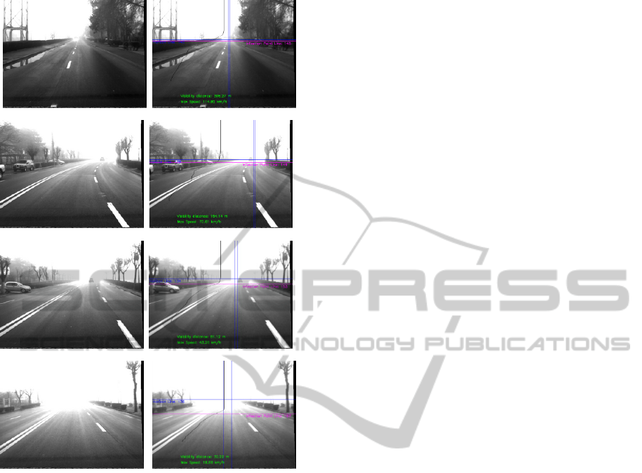
Figure 7 present the results of our fog detection

framework on real traffic images. These images

were acquired with a vehicle equipped with JAI-

A10-CL cameras during different fog conditions, in

the city of Cluj-Napoca. From top to bottom we

present different fog situations in accordance to the

fog categories presented in Table 1.

Table 3 presents the braking distances and the

necessary time for braking in the above four

scenarios. We can observe that the recommended

speed is accurate enough in order for the driver to

reduce the speed of the vehicle or even come to a

complete stop so as to avoid any collisions.

VISAPP2014-InternationalConferenceonComputerVisionTheoryandApplications

624

Original Image Fog Image: k = 0.03 Result Fog Image: k = 0.06 Result

Original Image Fog Image: k = 0.03 Result Fog Image: k = 0.09 Result

Original Image Fog Image: k = 0.06 Result Fog Image: k = 0.09 Result

Figure 6: Results obtained on synthetic images. The blue horizontal line represents the horizon line, the pink line represents

the inflection point line and the two vertical blue lines delimit the vertical band. The black curve represents the smoothed

median values from the vertical band .The visibility distances and the maximum recommended speeds are displayed in

green on the resulting images.

Table 3: Braking distance in the presented scenarios.

Fog

Scenario

Max

Speed

Braking

Distance

Braking

Time

km/h m s

1. Low Fog

114.95 148.62 4.65

2. Moderate Fog

70.61 56.08 2.86

3. Dense Fog

43.26 21.04 1.75

4.Very Dense Fog

18.88 4.01 0.76

Our algorithm was implemented in C++ and was

tested on an i7 based PC running Windows

operating system. The synthetic images have a

resolution of 688 x 515 pixels and the average

processing time is of 21 ms. The real traffic images

were obtained with a JAI CV-A10CL camera. Their

resolution is 512 x 383 pixels and the average

processing time on one image is 18 ms.

6 CONCLUSIONS

In this paper we have presented a framework for

detecting fog in images grabbed from a moving

vehicle with the goal of assisting the driver with safe

speed recommendations and information about the

fog density and visibility distance in order to avoid

accidents.

Our algorithm is able to detect fog on roads that

are not very crowded or when the field of view of

the ego vehicle’s camera is not occluded by other

vehicles. One of our main contributions is the

continuous estimation of the horizon line by using

the RANSAC method and the temporal integration

based on the consensus score. This approach proves

to be very stable and provides accurate results when

comparing to the estimation of the horizon line by

using only the camera parameters (obtained during

the offline calibration). By using the temporal

filtering based on the consensus score, we are able to

detect the horizon line even in tough scenarios

where the lane markings are not visible, during

curves, when the vehicle passes over speed bumps or

even in situation where the road is not flat. Another

important contribution is the temporal integration of

the inflection point line. This provides us with the

mean of estimating the density of the fog even in the

situations where we are not able to detect the vertical

band after the region growing process. Thus we are

still able to provide the driver with the maximum

speed recommendation on the given road segment.

The algorithm used to estimate the maximum

speed in fog situations proves to be accurate enough

in order for the driver to reduce the driving speed as

to avoid any collision with other traffic participants.

ACKNOWLEDGEMENTS

This work has been supported by UEFISCDI

(Romanian National Research Agency) in the

CELTIC+ research project Co-operative Mobility

Services of the Future (COMOSEF).

AssistingNavigationinHomogenousFog

625

Original Image Result (Low Fog)

Original Image Result (Moderate Fog)

Original Image Result (Dense Fog)

Original Image Result (Very Dense Fog)

Figure 7: Results obtained on real traffic images. The

visibility distance and the maximum recommended speed

are written on the resulting images.

REFERENCES

Berman, M., Liu, J. & Justison, L. 2009. Caltrans Fog

Detection and Warning System. White Paper, ICX

technologies.

Bota, S. & Nedevschi, S. 2006. GLSCENEINT: A

Synthetic image generation tool for testing computer

vision systems. Proceedings of IEEE 2nd

International Conference on Intelligent Computer

Communication and Processing, Cluj-Napoca,

Romania. pp.

Bronte, S., Bergasa, L. M. & Alcantarilla, P. F. 2009. Fog

detection system based on computer vision techniques.

12th International IEEE Conference on Intelligent

Transportation Systems. pp. 1-6.

Dong, N., Jia, Z., Shao, J., Li, Z., Liu, F., Zhao, J. & Peng,

P.-Y. 2011. Adaptive Object Detection and Visibility

Improvement in Foggy Image.

Enginneringtoolbox. The Engineering Toolbox [Online].

Available: http://www.engineeringtoolbox.com/

friction-coefficients-d_778.html.

Gallen, R., Hautiere, N. & Glaser, S. 2010. Advisory

speed for Intelligent Speed Adaptation in adverse

conditions. 2010 IEEE Intelligent Vehicles

Symposium. pp. 107-114.

Hautiere, N., Tarel, J.-P., Lavenant, J. & Aubert, D. 2006.

Automatic fog detection and estimation of visibility

distance through use of an onboard camera. Machine

Vision and Applications, 17, pp. 8-20.

Jimenez, F., Aparicio, F. & Paez, J. 2008. Evaluation of

in-vehicle dynamic speed assistance in Spain:

algorithm and driver behaviour. Intelligent Transport

Systems, IET, 2, pp. 132-142.

Middleton, W. 1952. Vision through the atmosphere,

Toronto: University of Toronto Press.

Mori, K., Kato, T., Takahashi, T., Ide, I., Murase, H.,

Miyahara, T. & Tamatsu, Y. 2006. Visibility

Estimation in Foggy Conditions by In-Vehicle Camera

and Radar. Innovative Computing, Information and

Control, 2006. ICICIC '06. First International

Conference on. pp. 548-551.

Negru, M. & Nedevschi, S. 2013. Image based fog

detection and visibility estimation for driving

assistance systems. Intelligent Computer

Communication and Processing (ICCP), 2013 IEEE

International Conference on. pp. 163-168.

Pavlic, M., Belzner, H., Rigoll, G. & Ilic, S. 2012. Image

based fog detection in vehicles. 2012 IEEE Intelligent

Vehicles Symposium pp. 1132-1137.

Pomerleau, D. 1997. Visibility estimation from a moving

vehicle using the RALPH vision system. IEEE

Conference on Intelligent Transportation System. pp.

906-911.

Se, S. 2000. Zebra-crossing detection for the partially

sighted. IEEE Conference on Computer Vision and

Pattern Recognition. pp. 211-217 vol.2.

VISAPP2014-InternationalConferenceonComputerVisionTheoryandApplications

626