Data Visualization using Decision Trees and Clustering
Olivier Parisot, Yoanne Didry, Pierrick Bruneau and Beno
ˆ
ıt Otjacques
Public Research Centre Gabriel Lippmann, Belvaux, Luxembourg
Keywords:
Data Visualization, Decision Tree Induction, Clustering.
Abstract:
Decision trees are simple and powerful tools for knowledge extraction and visual analysis. However, when
applied to complex datasets available nowadays, they tend to be large and uneasy to visualize. This difficulty
can be overcome by clustering the dataset and representing the decision tree of each cluster independently.
In order to apply the clustering more efficiently, we propose a method for adapting clustering results with a
view to simplifying the decision tree obtained from each cluster. A prototype has been implemented, and the
benefits of the proposed method are shown using the results of several experiments performed on the UCI
benchmark datasets.
1 INTRODUCTION
Originally used as a tool for decision support, deci-
sion trees are often used in data mining, especially
for classification (Quinlan, 1986). Moreover, they are
popular for the visual analysis of data (Barlow and
Neville, 2001; van den Elzen and van Wijk, 2011), be-
cause they use a formalism which is intuitive and easy
to understand for domain experts (Murthy, 1998).
From a dataset containing n features A
1
,...,A
n
, it
is possible to build a decision tree which explains the
value of the feature A
i
(often called class) according
to the values of the other features (A
j
( j 6= i)). This
model is a directed graph composed of nodes, leaves
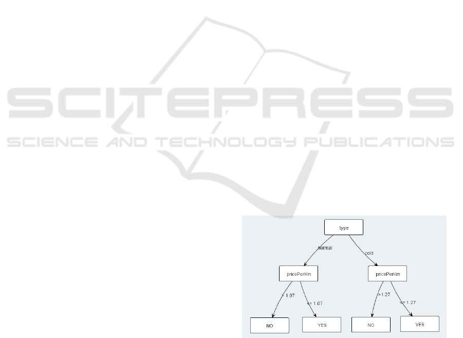
and branches. A node represents a feature, and each
node is followed by branches which specifiy a test on
the value of the feature (for instance: A
1
=’value’). A
leaf indicates a value of the class feature. From a
graphical point of view, decision trees are often repre-
sented using node-link diagrams (Figure 1), but other
representations like treemaps or concentric circles are
possible (Pham et al., 2008).
A decision tree obtained from data is character-
ized by two important properties: its complexity and
its accuracy regarding the data. The complexity of a
decision tree is often measured by its size, i.e. the
number of nodes (Breslow and Aha, 1997); neverthe-
less, others indicators such as tree width or tree depth
can be used. The accuracy of the tree is estimated us-
ing the error rate, i.e. the ratio of elements which are
not correctly explained using the tree (Breslow and
Aha, 1997). In order to obtain this error rate, a dataset
is often considered as two parts: the first one is used
to induce the decision tree (training set), and the sec-
ond one is used to compute the error rate (testing set).
But in order to obtain a decision tree which is repre-
sentative of the data, the whole dataset should rather
be used for both induction and error rate computation
(Parisot et al., 2013b).
Figure 1: A decision tree.
Decision tree induction has already been exten-
sively studied in the literature (Quinlan, 1986). The
main advantage of decision tree induction is that it
can be used with any kind of data, i.e. with nominal
and numeric features, and only the class feature has
to be discrete.
Unfortunately, real world datasets are traditionally
complex. As a result, the decision trees obtained from
these datasets are not always easily visualizable due to
their size or depth (Stiglic et al., 2012; Herman et al.,
1998).
Consequently, it is often useful to use other tech-
niques to obtain simpler decision trees. One of those,
clustering, allows to segment the data into homoge-
80
Parisot O., Didry Y., Bruneau P. and Otjacques B..
Data Visualization using Decision Trees and Clustering.
DOI: 10.5220/0004740800800087
In Proceedings of the 5th International Conference on Information Visualization Theory and Applications (IVAPP-2014), pages 80-87
ISBN: 978-989-758-005-5
Copyright
c
2014 SCITEPRESS (Science and Technology Publications, Lda.)
nous groups (called clusters). Decision trees may then
be built from each cluster.
In this work, we present a method that adapts the
clusters obtained from any clustering method, accord-
ing to the simplicity of the resulting decision trees.
The rest of this article is organized as follows.
Firstly, related works about simplification of decision
trees are discussed. Then, the presented method is de-
scribed in details. Finally, a prototype is presented,
and the results of experiments are discussed.
2 RELATED WORKS
Several methods have been proposed to simplify de-
cision trees obtained from data, with a minimal im-
pact on the decision trees accuracy (Breslow and Aha,
1997).
Firstly, pruning is a well-known solution to sim-
plify decision trees (Quinlan, 1987; Breslow and Aha,
1997). This technique removes the parts of the trees
which have a low explicative power (i.e. explaining
too few elements or with a high error-rate). More
specific pruning techniques allow to simplify decision
trees according to visual concerns: for instance, a re-
cent work has proposed a pruning technique which is
constrained by the dimensions of the produced deci-
sion tree (Stiglic et al., 2012), and another work has
described an algorithm to build decision tree with a
fixed depth (Farhangfar et al., 2008).
Secondly, decision tree simplification can be done
by working directly on the data, by using preprocess-
ing operations like feature selection and discretization
(Breslow and Aha, 1997). As these operations tend to
simplify the dataset (in term of dimensionality, num-
ber of possible values, etc.), they can also help to re-
duce the complexity of the associated decision tree (at
the expense of accuracy): this idea has been used in a
recent work (Parisot et al., 2013a).
Finally, clustering is a useful technique in data
mining, but it is also a promising tool in the context
of the visual analysis of data (Keim et al., 2008). A
priori, by splitting the data into homogenous groups,
it can be used to obtain simple decision trees. How-
ever, it is not always the case in practice. In fact, var-
ious methods of clustering exist (hierarchical, model-
based, center-based, search-based, fuzzy, etc.) (Gan
et al., 2007), but they often optimize a distance based-
criterion, with no account of the complexity of the
decision trees which are obtained from the clusters.
As a consequence, a recent solution has been pro-
posed to obtain a simple decision tree from each clus-
ter (Parisot et al., 2013b). Nevertheless, the algorithm
does not take into account the similarity between el-
ements and the dissimilartity between clusters: it is
not comparable to classic clustering results (obtained
with k-means, for example), and the results are hard
to interpret.
In this paper, we propose a solution to preserve in-
terpretability, by using existing clustering results as a
starting point, adapting these for simpler cluster-wise
decision trees, while maintaining good cluster quality
metrics.
3 CONTRIBUTION
In this section, we present a method to modify a clus-
tering result in order to simplify the decision tree spe-
cific to each cluster. In addition, the method guaran-
tees that the new clustering result is close to the initial
clustering result.
3.1 Adaptating a Clustering Result
The input of the proposed method is an initial clus-
tering result, which can be computed with any exist-
ing technique (k-means, EM, etc.) (Gan et al., 2007).
This result is then modified by an algorithm, which is
the core of our contribution.
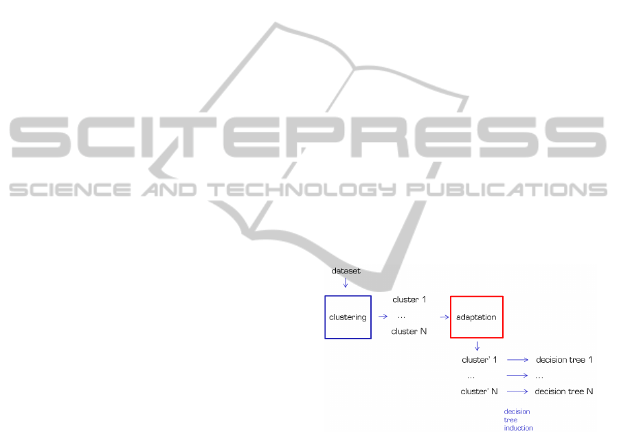
Figure 2: Clustering adaptation method.
In this work, we consider that adapting a cluster-
ing result C
1
,...,C
n
amounts to move elements from
C
i
to C
j
(i 6= j). In addition, we consider that finding
the cluster count, which is a complex problem (Wag-
ner and Wagner, 2007), is managed during the cre-
ation of the initial clustering result. Therefore, the
method does not modify the cluster count during the
clustering adaptation (in other words, no cluster is
created and/or deleted during the process).
3.2 Comparing with the Initial
Clustering Result
In order to guarantee that the modified clustering re-
sult is close to the initial clustering result, we use
DataVisualizationusingDecisionTreesandClustering
81

appropriate metrics. The literature contains a lot of
methods to compare two clustering results (Wagner
and Wagner, 2007); in this work, the Jaccard index is
used (Table 1) (Jaccard, 1908).
Table 1: Jaccard index definition.
E = initial clustering result
E’ = modified clustering result
N
11
= pairs in the same cluster in E and E’
N
10
= pairs in the same cluster in E,
not in the same cluster in E’
N
01
= pairs in the same cluster in E’,
not in the same cluster in E
Jaccard index = N
11
/(N
11
+ N
10
+ N
01
)
In practice, after the computation of the Jaccard
index between two clustering results, we obtain the
following behaviour:
• The more the Jaccard index is close to 1, the more
the two clustering results are similar.
• The more the Jaccard index is close to 0, the more
the two clustering results are dissimilar.
3.3 Algorithm
The adaptation is done using an algorithm (Algorithm
1) with the following inputs: a dataset with a class
feature, an initial clustering result, and a minimal Jac-
card index. The output is a new clustering result
where each cluster leads to a simpler decision tree.
The main idea of the algorithm is to incrementally
try to move the items between clusters in the limits
of a parameterized minimal Jaccard index. In pratice,
to handle the case when the minimal Jaccard index
isn’t reach, we define a maximal number of iterations
(when it does not find enough moves between clus-
ters).
The minimal Jaccard index has to be used as fol-
lows: specifying an index close to 1 amounts to con-
figure the algorithm to do few modifications, while
specifying an index close to 0 enables arbitrarily large
modifications.
The following sections explain how the moves be-
tween clusters are made.
3.4 Selecting the Items to Move
The goal is to modify the clusters in order to sim-
plify the decision tree of each cluster. As a result,
the items which are good candidates to be moved are
those which cause the decision tree complexity. We
have selected two kind of items:
Algorithm 1: Clustering adaptation algorithm.
Require:
0 < jaccardIndexLimit < 1
∧nbPassesLimit ≥ 0
Ensure:
nbPasses ← 0
j ← 1
while j < jaccardIndexLimit ∧ nbPasses <
nbPassesLimit do
for all item to mode do
search a target cluster C’ for item
if C’ exists then
move item into C’
j ←compute Jaccard index
end if
end for
nbPasses ← nbPasses + 1
end while
• The items badly classified/explained by the deci-
sion tree.
• The items explained by branches of the de-
cision tree having a low power of classifica-
tion/prediction.
A priori, it is reasonable to expect that moving
these items would not have a bad effect on the de-
cision tree generated from the initial cluster. In fact,
these items correspond to the tree branches which are
deleted by the classic pruning techniques.
A posteriori, for each element, it is important to
check if moving the item has really a good impact on
the decision tree generated from the initial cluster. To
do that, we compute the decision tree before moving
the item (DT), and the decision tree after moving the
item (DT’). Finally, we compare the complexity of
DT and DT’: if the size of DT’ is lower than the size
of DT, then the item can be moved.
3.5 Finding a Target Cluster
When an item has been selected as a good candidate to
be moved to another cluster, a target cluster has to be
found. To do that, we propose to select the cluster that
is the most favorably impacted by the inclusion of the
candidate. In other words, we compute the decision
tree for each cluster before adding the item (DT), and
the decision tree after adding the item (DT’); then we
compare the decision trees complexities. Two cases
can occur:
• If for each cluster, the size of DT’ is always higher
than the size of DT, than there is no target cluster:
the item is not moved.
IVAPP2014-InternationalConferenceonInformationVisualizationTheoryandApplications
82
• Else, the target cluster is the cluster for which the
ratio between the size of DT’ and the size of DT is
minimized: the item is moved to this target clus-
ter.
3.6 Usage of the Method
The method proposed by this paper aims at adapting
a clustering result to obtain clusters whith simpler de-
cision trees. This adapation is controlled by a param-
eter, the minimal Jaccard index, in order to obtain a
clustering result which is close to the original clus-
tering result. In other words, the parameter can be
useful to analyze data following the Visual Analytics
approach (Keim et al., 2008): adapted clustering re-
sults can be produced and refined in order to obtain
decision trees which are simple to analyse visually,
potentially shifting the clusters’ original meaning.
Yet, using an excessively low minimal Jaccard in-
dex is likely to harm cluster quality (e.g. high intra-
cluster similarity and low inter-cluster similarity). A
color-coded visual cue may indicate this danger to a
user.
4 EXPERIMENTS
In order to validate the approach described in this pa-
per, a prototype has been implemented and used on
several datasets. This section describes the prototype
and presents the experimental results.
4.1 Prototype
The prototype is a standalone tool implemented in
Java. It is based on Weka, a widely-used data mining
library (Hall et al., 2009), in order to use the imple-
mentations of the decision trees induction algorithm
and the k-means clustering algorithm. For the graph-
ical representation of the decision trees, the tool uses
Jung, a graphical library (O’Madadhain et al., 2003).
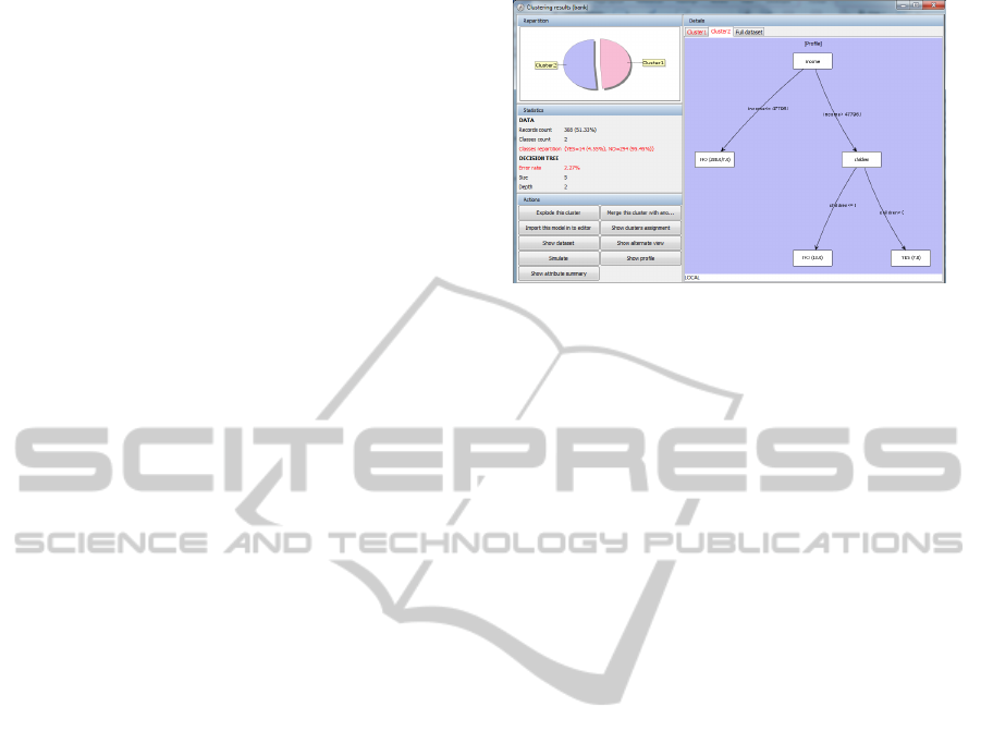
In addition to these building block components, the
prototype is completed with the implementation of
our clustering adaptation method, and with a graph-
ical user interface for the results exploration (statis-
tics about the datasets, graphical representation of the
clusters, etc. . . ) (Figure 3).
4.2 Test Procedure
Some tests have been performed on a selection of 10
well-known academic datasets (Bache and Lichman,
2013). This selection tries to cover several kinds of
Figure 3: Prototype.
datasets (number of records, features count, features
type, size and depth of decision trees, etc. . . ).
In order to check the impact of our method, for
each dataset we have compared the decision trees ob-
tained in the following cases:
• CASE 1: Decision tree induction on the full
dataset.
• CASE 2: Clustering with k-means (k=2,3,4), and
decision tree induction for each cluster.
• CASE 3: Clustering with k-means (k=2,3,4),
adaptation of the clustering result with our
method, and induction of the decision tree for
each cluster.
For the k-means clustering, the Euclidean distance
has been used. Moreover, the J48 algorithm has been
used to generate decision trees from data: it is a
widely used implementation of the C4.5 algorithm
(Quinlan, 1993). In practice, the J48 algorithm has to
be configured with several parameters; for these ex-
periments, we have disabled the ’pruning’ phase, in
order to initially obtain large decision trees and check
the benefits of our method.
4.3 Results
The experimental results (Tables 2,3,4) show the de-
cision trees obtained in the three cases previously de-
scribed. According to the case, the metrics are cho-
sen as follows: for CASE 1, we indicate the size and
the error rate of the decision tree generated from the
full dataset; for CASE 2 and CASE 3, we indicate the
mean sizes and error rates of the decision trees gen-
erated from the clusters. Moreover, we indicate for
CASE 3 the value of ji, the minimal Jaccard index
specified when running the adaptation method.
From these results, we can observe that it is pos-
sible to obtain simpler decision trees by simply using
a clustering technique like k-means, in comparison to
the decision trees obtained from the full dataset. For
instance, the dataset cmc leads to an initial decision
DataVisualizationusingDecisionTreesandClustering
83

Table 2: Results for 2 clusters. In CASE 1, we indicate the size and the error-rate for the full decision tree. In CASE 2 and 3,
we indicate the means of the sizes and the error-rates of the decision trees obtained from the clusters.
Dataset CASE 1 CASE 2 CASE 3 CASE 3 CASE 3 CASE 3
(full) (k-means) mji=0.95 mji=0.90 mji=0.85 mji=0.80
cmc 457/0.24 229/0.23 198/0.23 196/0.22 171/0.22 167/0.22
vehicle 173/0.06 71/0.07 53/0.11 51/0.09 50/0.09 n/a
autos 76/0.04 48/0.06 42/0.06 32/0.08 n/a n/a
credit-a 120/0.06 61/0.06 52/0.05 48/0.04 47/0.04 n/a
spectrometer 149/0.14 75/0.19 70/0.20 n/a n/a n/a
landsat 435/0.03 210/0.03 185/0.02 165/0.02 n/a n/a
credit-g 334/0.099 173/0.095 153/0.095 143/0.09 134/0.08 125/0.06
mushroom 47/0.33 95/0.33 61/0.33 n/a n/a n/a
anneal 59/0.009 37/0.005 26/0.004 n/a n/a n/a
bank-marketing 5120/0.04 2768/0.04 2246/0.03 1997/0.02 n/a n/a
adult 2442/0.09 1245/0.08 970/0.08 840/0.07 778/0.07 697/0.06
Table 3: Results for 3 clusters. In CASE 1, we indicate the size and the error-rate for the full decision tree. In CASE 2 and 3,
we indicate the means of the sizes and the error-rates of the decision trees obtained from the clusters.
Dataset CASE 1 CASE 2 CASE 3 CASE 3 CASE 3 CASE 3
(full) (k-means) mji=0.95 mji=0.90 mji=0.85 mji=0.80
cmc 457/0.24 57/0.13 49/0.12 37/0.11 37/0.10 31/0.10
vehicle 173/0.06 49/0.04 41/0.04 37/0.05 31/0.05 25/0.05
autos 76/0.04 30/0.06 25/0.06 21/0.09 n/a n/a
credit-a 120/0.06 40/0.05 27/0.03 27/0.03 25/0.03 20/0.02
spectrometer 149/0.14 51/0.16 47/0.16 43/0.18 41/0.18 41/0.16
landsat 435/0.03 75/0.02 53/0.02 n/a n/a n/a
credit-g 334/0.10 108/0.08 98/0.07 91/0.06 80/0.05 74/0.06
mushroom 47/0.33 16/0.26 16/0.25 16/0.23 n/a n/a
anneal 59/0.009 19/0.003 18/0.001 n/a n/a n/a
bank-marketing 5120/0.04 1916/0.04 1492/0.03 1347/0.02 1158/0.02 n/a
adult 2442/0.09 391/0.07 308/0.06 260/0.04 231/0.03 188/0.01
Table 4: Results for 4 clusters. In CASE 1, we indicate the size and the error-rate for the full decision tree. In CASE 2 and 3,
we indicate the means of the sizes and the error-rates of the decision trees obtained from the clusters.
Dataset CASE 1 CASE 2 CASE 3 CASE 3 CASE 3 CASE 3
(full) (k-means) mji=0.95 mji=0.90 mji=0.85 mji=0.80
cmc 457/0.24 78/.18 57/.20 48/.19 42/.19 37/.19
vehicle 173/0.06 10/.01 7/.01 5/.01 n/a n/a
autos 76/0.04 24/.10 20/.09 16/.10 n/a n/a
credit-a 120/0.06 24/.04 21/.06 18/.04 n/a n/a
spectrometer 149/0.14 39/.19 37/.19 34/.20 n/a n/a
landsat 435/0.03 53/.02 39/.02 32/.01 n/a n/a
credit-g 334/0.10 71/.09 50/.09 47/.08 45/.06 n/a
mushroom 47/0.33 64/.31 37/.31 n/a n/a n/a
anneal 59/0.009 22/.01 19/.00 n/a n/a n/a
bank-marketing 5120/0.04 1375/.05 1168/.04 971/.03 850/.02 n/a
adult 2442/0.09 438/.09 370/.08 318/.07 279/.05 254/.04
tree with a size of 457, and using the k-means algo-
rithms allows to obtain decisions trees with a mean
size of 229 for 2 clusters and 57 for 3 clusters. In
addition, the results show that our clustering adapta-
tion method significantly simplifies the decision trees
of the clusters. For the dataset cmc, our technique
allows to reduce the mean size of the decision trees:
up to 27% for 2 clusters, and up to 46% for 3 clus-
IVAPP2014-InternationalConferenceonInformationVisualizationTheoryandApplications
84
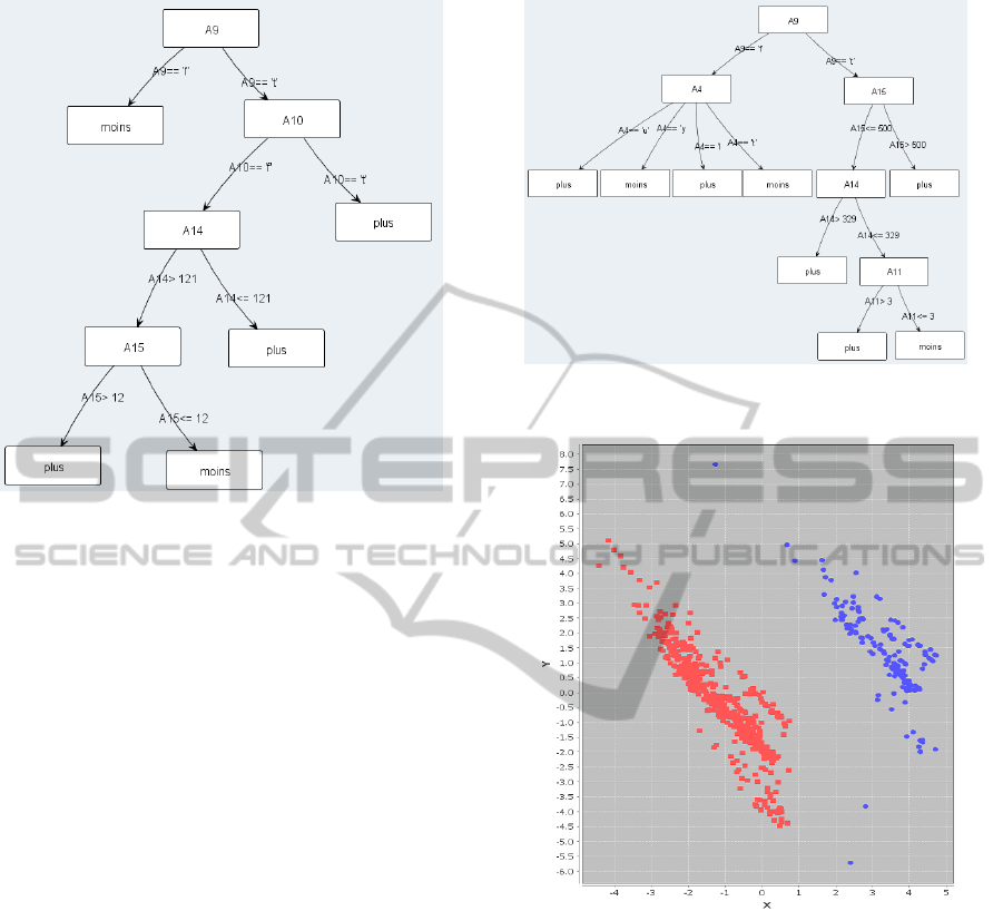
Figure 4: ’credit-a’ clustered with k-means (k=2) and
adapted with our method: the first cluster’s decision tree.
ters. The most important gains are observed for the
vehicle, credit-a, and adult datasets: in these cases,
the mean sizes of the decision trees for the clusters
can be reduced up to 50% for 3 clusters. But it is
not always so efficient: in some cases (like mush-
room split in 3 clusters), k-means produces clusters
for which decision trees are very simple: our method
hardly simplifies them further. It is important to say
that the decision trees obtained with our method do
not lose accuracy: the computed error rates tend to
decrease. By comparison, the classical decision tree
simplification methods tend to produce decision trees
with higher error rates (Breslow and Aha, 1997).
Finally, the results show that for the majority of
the tested datasets, it is not possible to drop below a
certain value of Jaccard index (the most significative
case is spectrometer, 2 clusters): it means that after
a certain count of moves, the algorithm can not find
others moves which can simplify decision trees. It is
not a problem, because our method aims to provide
clustering results which globally keep the meaning of
the original clustering results.
4.4 Impact for Decision Trees
Visualization
The method presented in this paper allows to sim-
plify decision trees by adapting clustering results. If
we combine this method with existing pruning tech-
niques, we can obtain decision trees which are simple
to visualize. For instance, the credit-a dataset leads
to a decision tree with a size of 63 by using the J48
Figure 5: ’credit-a’ clustered with k-means (k=2) and
adapted with our method: the second cluster’s decision tree.
Figure 6: PCA projection for ’credit-a’, colored using k-
means (k=2): the x axis represents the first principal com-
ponent, and the y axis represents the second principal com-
ponent.
induction algorithm with pruning enabled. And if we
apply our method by setting the minimum Jaccard in-
dex to 0.9, we obtain two clusters with simpler deci-
sion trees (sizes=9 and 13), which are easily visualiz-
able (Figures 4,5).
4.5 Impact on the Clustering Results
It can be useful to show the impact of our adap-
tation method on the clustering results: to do that,
well-known cluster interpretation methods like pro-
jections can be used (Gan et al., 2007). For the credit-
a dataset, a PCA projection (Principal Component
Analysis) allows to show that the clusters are less
DataVisualizationusingDecisionTreesandClustering
85
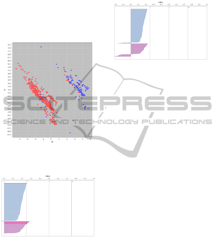
correct after adaptation (Figures 6,7), as confirmed
by a Silhouette plot (Figures 8,9) (Rousseeuw, 1987).
The clustering results are less correct, but the decision
trees are simpler: so our method allows to influence
the tradeoff between simplicity of decision trees and
similarity with the initial clustering.
Figure 7: PCA projection for ’credit-a’, colored with k-
means (k=2) adapted with our method (minimum Jaccard
index=0.9): the x axis represents the first principal compo-
nent, and the y axis represents the second principal compo-
nent.
Figure 8: Silhouette plot for ’credit-a’, using k-means clus-
tering(k=2): the x axis represents the Silhouette value, and
the y axis represents the elements (sorted by clusters and
Silhouette values). In practice: larger Silhouette values in-
dicate a better quality of the clustering result.
5 CONCLUSIONS
We presented a method based on clustering and deci-
sion tree induction that optimize the visual represen-
Figure 9: Silhouette plot for ’credit-a’, using k-means (k=2)
adapted with our method (minimum Jaccard index=0.9):
the x axis represents the Silhouette value, and the y axis
represents the elements (sorted by clusters and Silhouette
values). In practice: larger Silhouette values indicate a bet-
ter quality of the clustering result.
tation of complex datasets. This method proceeds by
modifying a clustering result to obtain simpler deci-
sion trees for all clusters. The method has been im-
plemented in a prototype, and its effectiveness was
demonstrated on well-known UCI datasets.
We are now adapting the solution in order to sup-
port data streams, by using incremental decision trees
induction methods and stream clustering algorithms.
Moreover, we have in view to extend the method by
using other heuristics such as genetic algorithms.
REFERENCES
Bache, K. and Lichman, M. (2013). UCI machine learning
repository.
Barlow, T. and Neville, P. (2001). Case study: Visualization
for decision tree analysis in data mining. In Proceed-
ings of the IEEE Symposium on Information Visualiza-
tion 2001 (INFOVIS’01), INFOVIS ’01, pages 149–,
Washington, DC, USA. IEEE Computer Society.
Breslow, L. A. and Aha, D. W. (1997). Simplifying decision
trees: A survey. Knowl. Eng. Rev., 12(1):1–40.
Farhangfar, A., Greiner, R., and Zinkevich, M. (2008). A
fast way to produce optimal fixed-depth decision trees.
In ISAIM.
Gan, G., Ma, C., and Wu, J. (2007). Data clustering - the-
ory, algorithms, and applications. SIAM.
Hall, M., Frank, E., Holmes, G., Pfahringer, B., Reute-
mann, P., and Witten, I. H. (2009). The weka data
mining software: an update. SIGKDD Explor. Newsl.,
11(1):10–18.
Herman, I., Delest, M., and Melancon, G. (1998). Tree vi-
sualisation and navigation clues for information visu-
alisation. Technical report, Amsterdam, The Nether-
lands, The Netherlands.
Jaccard, P. (1908). Nouvelles recherches sur la distribution
florale. Bulletin de la Soci
´
et
´
e vaudoise des sciences
naturelles. Impr. R
´
eunies.
IVAPP2014-InternationalConferenceonInformationVisualizationTheoryandApplications
86

Keim, D., Andrienko, G., Fekete, J.-D., G
¨
org, C., Kohlham-
mer, J., and Melanc¸on, G. (2008). Information vi-
sualization. chapter Visual Analytics: Definition,
Process, and Challenges, pages 154–175. Springer-
Verlag, Berlin, Heidelberg.
Murthy, S. K. (1998). Automatic construction of decision
trees from data: A multi-disciplinary survey. Data
Min. Knowl. Discov., 2(4):345–389.
O’Madadhain, J., Fisher, D., White, S., and Boey, Y. (2003).
The JUNG (Java Universal Network/Graph) frame-
work. Technical report, UCI-ICS.
Parisot, O., Bruneau, P., Didry, Y., and Tamisier, T. (2013a).
User-driven data preprocessing for decision support.
In Luo, Y., editor, Cooperative Design, Visualization,
and Engineering, volume 8091 of Lecture Notes in
Computer Science, pages 81–84. Springer Berlin Hei-
delberg.
Parisot, O., Didry, Y., Tamisier, T., and Otjacques, B.
(2013b). Using clustering to improve decision trees
visualization. In Proceedings of the 17th Inter-
national Conference Information Visualisation (IV),
pages 186–191, London, United Kingdom.
Pham, N.-K., Do, T.-N., Poulet, F., and Morin, A. (2008).
Treeview, exploration interactive des arbres de dci-
sion. Revue d’Intelligence Artificielle, 22(3-4):473–
487.
Quinlan, J. R. (1986). Induction of decision trees. Machine
Learning, 1:81–106.
Quinlan, J. R. (1987). Simplifying decision trees. Int. J.
Man-Mach. Stud., 27(3):221–234.
Quinlan, J. R. (1993). C4.5: programs for machine learn-
ing. Morgan Kaufmann Publishers Inc., San Fran-
cisco, CA, USA.
Rousseeuw, P. J. (1987). Silhouettes: a graphical aid to
the interpretation and validation of cluster analysis.
Journal of computational and applied mathematics,
20:53–65.
Stiglic, G., Kocbek, S., Pernek, I., and Kokol, P. (2012).
Comprehensive decision tree models in bioinformat-
ics. PLoS ONE, 7(3):e33812.
van den Elzen, S. and van Wijk, J. (2011). Baobabview:
Interactive construction and analysis of decision trees.
In Visual Analytics Science and Technology (VAST),
2011 IEEE Conference on, pages 151–160.
Wagner, S. and Wagner, D. (2007). Comparing clusterings:
an overview. Universit
¨
at Karlsruhe, Fakult
¨
at f
¨
ur In-
formatik.
DataVisualizationusingDecisionTreesandClustering
87
