
Statistical Features for Image Retrieval
A Quantitative Comparison
Cecilia Di Ruberto and Giuseppe Fodde
Department of Mathematics and Computer Science, University of Cagliari, via Ospedale 72, 09124 Cagliari, Italy
Keywords:
Texture, Feature Extraction, Feature Selection, Classification, Statistical Texture Analysis.
Abstract:
In this paper we present a comparison between various statistical descriptors and analyze their goodness in
classifying textural images. The chosen statistical descriptors have been proposed by Tamura, Battiato and
Haralick. In this work we also test a combination of the three descriptors for texture analysis. The databases
used in our study are the well-known Brodatz’s album and DDSM (Heath et al., 1998). The computed features
are classified using the Naive Bayes, the RBF, the KNN, the Random Forest and Random Tree models. The
results obtained from this study show that we can achieve a high classification accuracy if the descriptors are
used all together.
1 INTRODUCTION
Texture analysis is a process that allows the character-
ization of different surfaces and objects by identifying
their specific statistical properties. Through rigorous
techniques of image capture, you can get a texture on
a given surface that uniquely identifies its structure
depending on the lighting and the intensity captured
during acquisition. From this it’s possible to extract
characteristics or features that allow the actual im-
age texture characterization, by means of an adequate
mathematical formulation. In this experimental anal-
ysis we compare three types of statistical descriptors
that define, although in a different way, the same fea-
tures: coarseness, contrast and directionality accord-
ing to Battiato’s (Battiato et al., 2003) and Tamura’s
(Tamura et al., 1978) definitions and contrast, energy
and entropy making use the co-occurrence matrices as
defined by Haralick (Haralick, 1979). The analysis is
achieved in two different phases: in the first one there
is the features extraction through the descriptors cal-
culation and in the second one the calculated data are
classified using five classifiers: the Naive Bayes, the
RBF, the k-Nearest Neighbor, the Random-Forest and
Random-Tree. The classification is also performed
using a feature selection process. The experimental
study has been applied on the well-know database of
Brodatz’s album and on DDSM (Heath et al., 1998),
a mammographic images database. The results ob-
tained with this experimental analysis have led to ob-
tain a high percentage of instances correctly classified
if we use the descriptors all together, both with and
without a feature selection, by using all the classifi-
cation models. The rest of the paper is organized as
follows: in section 2 theconsidered statistical descrip-
tors are illustrated in details, in Section 3 we explain
our comparison study, in Section 4 we illustrate the
results obtained and, finally, in Section 5 we have the
conclusions.
2 THREE BASIC STATISTICAL
DESCRIPTORS
In literature there are several methods used for feature
extraction from textured images, each of them based
on a different type of texture (Rosenfeld, 1975) (van
den Broek and Rikxoort, 2004) (Broek and Rikxoort,
2005). In Image Processing the term texture refers to
any and repetitive geometric arrangement of the gray
levels of an image (Broek and Rikxoort, 2005). The
texture provides important information about the spa-
tial arrangement of the gray levels and their relation-
ship with the surrounding elements. The human vi-
sual system determines and easy recognizes different
types of texture characterizing them in a subjective
way but, even if for a human observer it is simple and
intuitive to associate with a surface texture a partic-
ular concept, give a strict definition of what is very
difficult (van Rikxoort et al., 2005). In fact, there is
no general definition of texture and a methodology for
610
Di Ruberto C. and Fodde G..
Statistical Features for Image Retrieval - A Quantitative Comparison.
DOI: 10.5220/0004741006100617
In Proceedings of the 9th International Conference on Computer Vision Theory and Applications (VISAPP-2014), pages 610-617
ISBN: 978-989-758-003-1
Copyright
c
2014 SCITEPRESS (Science and Technology Publications, Lda.)

Figure 1: Textured images examples: on the left Brodatz’s
image and on the right DDSM’s image.
measuring the texture accepted by all. We can see ex-
amples of textured images in Fig. 1. Texture analysis
has three fundamental aspects like classification, seg-
mentation and shape from texture which determines
regions of texture among different predefined classes
of texture, the boundaries between regions with dif-
ferent textures and the reconstruction of the surface
objects starting from different kind of texture, respec-
tively. For texture analysis we can use a statistical
approach which includes the statistics of the first, sec-
ond and high order. Among the various methods for
a statistical perceptual texture analysis we consider
three simple and fast approaches (Prasad and Krishna,
2011). The first of these has been proposedby Tamura
(Tamura et al., 1978) and explains how to calculate
six texture features (coarseness, contrast, directional-
ity, line-likeness, regularity and roughness) of which
only the first three are actually being used. The lat-
ter in fact turn out to be redundant and not more dis-
criminating than the former. The second one has been
proposed by Battiato (Battiato et al., 2003) that gives
a different definition of the same texture features of
Tamura. The last one has been proposed by Haralick
(Haralick, 1979) and we consider in particular three
features among the fourteen defined: contrast, energy
and entropy.
2.1 Tamura’s Descriptors
Tamura’s features are extracted from texture descrip-
tors that correspond to human visual perception. Six
features are extracted but only the first three are con-
sidered in subsequent studies because the last three do
not add relevant information. The Tamura’s features
try to give a numerical value to each texture taken
into consideration in order to relate the results with
the human visual perception. The features extracted
are: coarseness, contrast, directionality, line-likeness,
regularity and roughness.
Coarseness: it is a fundamental texture feature and
can be defined as the granularity. When two pat-
terns differ only in the scale, the pattern appears larger
coarse. If you have patterns with different structures,
a coarse texture contains a small number of large el-
ements, while a fine texture contains a large number
of small elements. The higher coarseness value repre-
sents a fine texture. The essence of this method is to
pick a large size as best when coarse texture is present
even though micro-texture is also present but to pick a
small size when only fine texture is present. To com-
pute this feature it is possible to follow a procedure
summarized in the following steps.
• Step 1. Take averages at every point over neigh-
borhoods whose sizes are powers of two. The av-
erage over the neighborhood of size 2
k
∗2
k
at the
point (x,y) is:
A
k
(x,y) =
x+2
k−1
−1
∑
i=x−2
k−1
y+2
k−1
−1
∑
j=y−2
k−1
f(i, j)/2
2k
(1)
where f(i, j) is the gray level at (i,j).
• Step 2. For each point, take differences between
pairs of averages corresponding to pairs of non-
overlapping neighborhoods just on opposite sides
of the point in both horizontal and vertical orien-
tations. For example, the difference in the hori-
zontal case is
E
k,h
(x,y) = |A
k
(x+ 2
k−1
,y) − A
k
(x− 2
k−1
,y)|
(2)
• Step 3. At each point, pick the best size which
gives the highest output value:
S
best
(x,y) = 2
k
(3)
• Step 4. Finally, take the average of S
best
over the
picture to be a coarseness measure F
crs
:
F
crs
=
1
m∗ n
m
∑
i
n
∑
j
S
best
(i, j) (4)
where m∗ n is the image dimension.
Contrast: this feature is influenced by several fac-
tors: the range of gray levels, the relationship between
black and white between the texture areas, the sharp-
ness of the edges and the frequency of repetition of
the plot. It can be said that the contrast is synony-
mous of image quality. To calculate the contrast we
need the measure of kurtosis that can be defined as:
α
4
=
µ
4
σ
4
(5)
where µ
4
is the fourth moment about the mean and σ
2
is the variance. Combining σ and α
4
we obtain the
measure of contrast as follows:
F
con
=
σ
(α
4
)
n
(6)
StatisticalFeaturesforImageRetrieval-AQuantitativeComparison
611

where n is a positive number.
Directionality: it is a global property of the region
of interest. Tamura measures the overall degree of
directionality where the orientation of the pattern of
the texture does not matter. Tamura uses a histogram
of local edge against their directional angle. This his-
togram is sufficient to describe the overallcharacteris-
tics of the input image as long lines and simple curves.
The method uses the fact that the gradient is a vec-
tor and has both a magnitude and a direction. The
approach proposed by Tamura is to sum the second
moments around each pick from valley to valley, if
multiple peaks are determined to exist. This measure
can be defined as follows:
F
dir
= 1 − r ∗ n
p
∗
n
p
∑
p
∑
φ∈w
p
(φ− φ
2
) ∗ H
D
(φ) (7)
where n
p
is the number of peaks, r is a normalizing
factor related to quantizing levels of φ and φ is a quan-
tized direction code. H
D
is the desired histogram de-
fined as follows:
H
D
(k) = N
θ
(k)/
n−1
∑
i=0
N
θ
(i) (8)
where N
θ
(i) is the number of points and k =
0,1,...,n− 1.
The other three features of Tamura are defined as fol-
lows.
Line-likeness is a feature that only affects the shape
of the elements of the texture, it means all those el-
ements which are composed of lines. In this case,
when the direction of an edge and the direction of the
neighbors edges are almost equal, it considers an edge
points group as a line.
Regularity is calculated considering the variation of
the elements. It is assumed, in fact, that the variations
of the elements, especially in the case of natural tex-
ture, reduce the regularity in the complex. In addition,
it can be said that a fine texture tends to be perceived
as smooth. If any texture feature varies across the im-
age, then the same is irregular.
Roughness indicates the roughness of a texture. It’s
a typical feature of tactile textures rather than visual.
The effects of coarseness and contrast are emphasized
and a measure of the roughness is approximated using
these features.
2.2 Battiato’s Descriptors
In (Battiato et al., 2003) Battiato proposes a variant to
Tamura’s features based on the calculation of the co-
occurrence matrices. Battiato presents a visual sys-
tem that starting from graphical cues representing rel-
evant perceptual texture features, interactively looks
more like those in a set of candidates belonging to
the same space texture. Textures are described us-
ing mathematical models and purely statistical fea-
tures that allow you to perform a classification both
supervised and not supervised. The alternative ap-
proach is to identify and measure the features con-
sidered most relevant to human perception (van den
Broek et al., 2006). The features proposed are the
first three of Tamura: coarseness, contrast and direc-
tionality according to local properties. These features
are used to produce a ”perceptual space” where multi-
dimensional textures are organized according to the
axes of perception. The features calculated can be
used to create a visual system for navigation and re-
trieval in large texture database. Then iconic repre-
sentations are created and used to formulate a query
to search for interactive visual texture through the hu-
man perceptual qualities. The three features proposed
are defined as follows.
Coarseness: it is probably the most essential percep-
tual feature, in fact many times, the word ”coarse-
ness” coincides with ”texture”. The coarseness de-
fines the granularity of the image. It is calculated us-
ing an algorithm that has four steps:
• Step 1: K images are created in which each ele-
ment is the average of the intensities between the
neighbors:
A
k
(x,y) =
1
2
2k
∗
x+2
k−1
−1
∑
i=x−2
k−1
y+2
k−1
−1
∑
j=y−2
k−1
f(i, j) (9)
• Step 2: take the differences between the pairs of
averages that correspond to the area that does not
overlap either horizontally or vertically:
E
k,horiz
(x,y) = |A
k
(x+ 2
k−1
,y) − A
k
(x− 2
k−1
,y)|
(10)
E
k,vert
(x,y) = |A
k
(x,y+ 2
k−1
) − A
k
(x,y− 2
k−1
)|
(11)
• Step 3: for each pixel the maximum difference
between adjacent regions is calculated:
S
best
(x,y) = k (12)
where k maximizes the differences:
E
k
= max(E
k,horiz
,E
k,vert
) (13)
• Step 4: calculate the value of the global coarse-
ness:
coarseness =
1
m∗ n
m
∑
j=1
n
∑
i=1
S
best
(i, j). (14)
Contrast: this measure is based on the calculation
of the local contrast defined for each pixel with the
VISAPP2014-InternationalConferenceonComputerVisionTheoryandApplications
612

estimation of the local variation in the neighborhood
of the neighbors. Local contrast is commonly defined
for each pixel as an estimate of the local variation in a
neighborhood. Given a pixel p = (i, j) and a neighbor
mask W ∗ W of the pixel, local contrast is computed
as:
local contrast(i, j) =
max
p∈W∗W
(p) − min
p∈W∗W
(p)
min
p∈W∗W
(p) + max
p∈W∗W
(p)
(15)
The global contrast is defined as the global arithmetic
mean of all the local contrast values over the image:
contrast =
1
m∗ n
∗
m
∑
j=1
n
∑
i=1
local
contrast(i, j) (16)
where m∗ n is the image dimension.
Directionality: this measure is based on Haralick co-
occurrence matrices. Their computation is focused on
the calculation of the degree of confidence for a given
orientation of the texture. In other words, instead of
calculating a global value of directionality, is calcu-
lated a ”degree of confidence of significance” for a
set of guidelines.
Let T be a texture of size m∗n∗c colors and ν(x, y)
an offset vector, the co-occurrence matrix C(T,ν) is a
c∗ c matrix defined in each point by:
C(T,ν)
i, j
= |(p, q) in T ∗ T : q = p+ ν,
L(p) = i,L(q) = j|
(17)
where L(p) is the luminance value of the pixel p.
Then a point (i, j) in C contains the number of pix-
els pairs in T that have respectively gray level i and j
and with displacement vector ν. The measure pro-
posed in the paper is based on a simple idea: the plot
of the main diagonal of a co-occurrence matrix with
offset ν is closer to the histogram of the image as ν is
relative to a relevant direction.
2.3 Haralick’s Descriptors
In (Haralick, 1979) it has been implemented a method
of content-based image retrieval (CBIR) for medi-
cal imaging, alternative and complementary to that
based on the use of keywords. This system is based
on the effective use of information of the texture of
the images. The system is also part of the so-called
computer-aided diagnosis systems (CAD) that help
doctors make better decisions in the shortest possible
time thus promoting early diagnosis. Three specific
features are extracted: energy, contrast and entropy.
These features are calculated using the co-occurrence
matrices, computed for various angular relationships
and distances between pairs of neighboring cells of
the image.
Energy: it is also known as uniformityor angular sec-
ond moment. It assumes the value of zero if the image
is constant. Energy is defined as follows:
energy =
∑
i
∑
j
c(i, j)
2
(18)
where c(i, j) is the value of co-occurrence matrix in
(i, j).
Contrast: it is the weighted average of all diagonals
parallel to the main one that rewards more and more
remote from the latter. Its value is zero if the image is
constant. Contrast is defined as follows:
contrast =
N
g−1
∑
n=0
n
2
{
N
g
∑
i=1
N
g
∑
j=1
c(i, j)} (19)
where |i− j| = n.
Entropy: it expresses the measure of the entropy of
the matrix in its entirety. Entropy is defined as fol-
lows:
entropy = −
∑
i
∑
j
c(i, j)log(c(i, j)). (20)
3 OUR COMPARISON STUDY
In this work we compare the previous features de-
scriptors for classification of textured images, taken
from the Brodatz’s album (Brodatz, 1966) and DDSM
(Heath et al., 1998) and we analyze the goodness
of classification obtained by combining them, too.
The proposed comparison is developed in two main
phases: in the first there is the texture features extrac-
tion, while in the second one there is the images clas-
sification by using the descriptors calculated in the
previous phase. Various datasets are generated, each
containing various combinations of descriptors: at the
beginning the three types of descriptors are taken in-
dividually, then they are taken in pairs of two and fi-
nally combined all together. Before the classification
phase a feature selection step has been introduced.
3.1 Feature Extraction
In this first phase the features for the three types of
descriptors are calculated. We obtain a features vec-
tor that varies from a minimum of nine to a maxi-
mum of eighteen depending on the number of angles
of the co-occurrences matrix that we decide to con-
sider: three are related to Tamura’s features (coarse-
ness, contrast and directionality), three to Battiato’s
features (coarseness, contrast and directionality) and
three to twelveare relativeto Haralick’s features (con-
trast, energy and entropy). In extracting Haralick’s
StatisticalFeaturesforImageRetrieval-AQuantitativeComparison
613
features, initially we calculate the co-occurrence ma-
trix using only one angle, that of orientation 0
◦
and
with distance equal to one, thus obtaining only three
features. Then we modify the offset for the calcula-
tion of co-occurrence matrix adding the other three
angles of the upper part of the image: 0
◦
, 45
◦
, 90
◦
and 135
◦
. Finally, the offset has been modified further
to include all the eight possible angles: 0
◦
, 45
◦
, 90
◦
,
135
◦
, 180
◦
, 225
◦
, 270
◦
and 315
◦
. After generating
the co-occurrence matrix, we evaluate the properties
related to it, going to keep only the energy, contrast
and entropy to be used in the classification.
3.2 Feature Selection
This phase is carried out after an initial phase of clas-
sification to see if the results already obtained could
be further improved. It is carried out a selection of at-
tributes by ranking the positive values of the correla-
tion with the class attribute in descending order. This
phase has led to improvements of classification accu-
racy, even of 7-8%. However, in very few cases no
attributes have been eliminated but a different rank-
ing of them has produced a worsening of classifica-
tion, as happened with the Random Forest classifier.
Also during this phase, the more frequently discarded
attribute is the Battiato’s contrast.
3.3 Classification
The classification stage is the last of this experimen-
tal study. For this phase we use five different types of
classifiers: Naive Bayes, RBF, k-NN, Random Forest
and Random Tree. We decide to use the technique of
ten fold cross-validation where the original dataset is
divided into subsets each consisting of the same num-
ber of samples (ten in this case). The data are first
classified by analyzing the original dataset (i.e. with-
out feature selection) and then by applying the same
classifiers after the feature selection step.
4 EXPERIMENTAL RESULTS
Now we present the numerical results obtained using
the illustrated texture descriptors in classifying two
different datasets: the well known Brodatz album and
the DDSM (Heath et al., 1998). The DDSM contains
a series of mammography screenings stored in four
different categories: Normal, Cancer, Benign, Benign
Without Callback. In both the experiments we show
the accuracy values using the three descriptors indi-
vidually, then combined in pairs and finally combined
all together. A set of forty images taken from Bro-
datz’s album is used, which has been divided into four
non-overlappingportions of equal size; while for each
category of DDSM we use twenty different images.
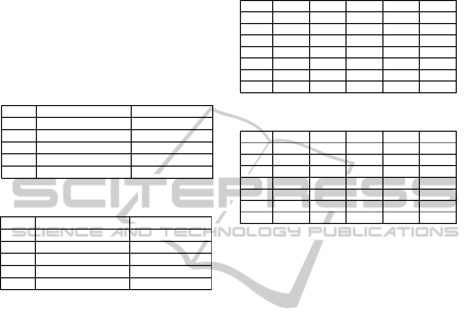
4.1 By Tamura’s Descriptors on
Brodatz Album
In Table 1 we present the results by using Tamura’s
features, with and without feature selection. In this
case the highest accuracy value is achieved already
before the feature selection with 81.5% of the RBF
classifier, also confirmed after the feature selection.
Table 1: Results by using Tamura’s features, with and with-
out feature selection.
No feature selection Feature selection
NB 75.3% 81.5%
RBF 81.5% 81.5%
KNN 73.5% 73.5%
R-F 71.5% 71.5%
R-T 70.9% 70.9%
4.2 By Battiato’s Descriptors on
Brodatz Album
Let’s see in Table 11 the results obtained by Bat-
tiato’s features. By using the original dataset, the best
accuracy is achieved with the RBF that goes up to
79.6% of instances correctly classified. After the fea-
ture selection the classification improves touching the
threshold of 80.8% accuracy obtained with the KNN.
Table 2: Results by using Battiato’s features, with and with-
out feature selection.
No feature selection Feature selection
NB 78.8% 82.4%
RBF 79.6% 80.5%
KNN 63.6% 80.8%
R-F 61.4% 73%
R-T 68.7% 72.3%
4.3 By Haralick’s Descriptors on
Brodatz Album
Let’s see now the results obtained with only one ori-
entation angle in Table 3. The results obtained with
these descriptors are good even without the feature
selection, reaching 81.4% of instances correctly clas-
sified. After the feature selection the accuracy is
slightly uphill coming up to 82.3% with Random For-
est classifier.
VISAPP2014-InternationalConferenceonComputerVisionTheoryandApplications
614

Now let’s see the classification using the four an-
gles in Table 4. As we can see from the table the best
result without feature selection is 89.5%, while this
value after the feature selection comes down and the
best is 88.8%. This is related to a different attributes
ranking during the classification.
Table 3: Results by using Haralick’s features with one an-
gle, with and without feature selection.
No feature selection Feature selection
NB 77.1% 77.1%
RBF 68.7% 74.1%
KNN 77.8% 77.8%
R-F 81.4% 82.3%
R-T 76.7% 80%
Table 4: Results by using Haralick’s features with four an-
gles, with and without feature selection.
No feature selection Feature selection
NB 87.4% 87.4%
RBF 88.8% 88.8%
KNN 87% 87%
R-F 89.5% 77.5%
R-T 78.9% 85.7%
4.4 By Battiato’s and Tamura’s
Descriptors on Brodatz Album
The first combination of descriptors is between the
different definitions of Tamura’s features.
Let’s see the accuracy percentages obtained in Ta-
ble 5. The accuracy is already high without feature
selection with a peak of 92.2% achieved with KNN.
After the attributes selection we still have the highest
accuracy with the same classifier.
Table 5: Results by using Battiato’s and Tamura’s features,
with and without feature selection.
No feature selection Feature selection
NB 89.3% 94%
RBF 88.4% 95.9%
KNN 92.2% 100%
R-F 80.5% 94.4%
R-T 69.5% 92.6%
4.5 By Battiato’s and Haralick’s
Descriptors on Brodatz Album
In this experimentation we combine the features pro-
posed by Battiato and those of Haralick using the co-
occurrence matrix with the four corners of the upper
part of the image.
Let’s see the results in Table 6. Before the fea-
ture selection, the classifiers performing better are the
Bayesian and the KNN, arriving both at 86.4% of in-
stances correctly classified while after feature selec-
tion the best is always the KNN with an accuracy of
95.3%.
Table 6: Results by using Battiato’s and Haralick’s features,
with and without feature selection.
No feature selection Feature selection
NB 86.4% 92.8%
RBF 86% 93.2%
KNN 86.4% 95.3%
R-F 84.5% 91.3%
R-T 79.4% 76.1%
4.6 By Tamura’s and Haralick’s
Descriptors on Brodatz Album
The last combination of two types of descriptors is
between Tamura’s and Haralick’s features.
The accuracy values obtained are showed in Ta-
ble 7. Also in this case the feature selection does not
affect the best result that, both before and after, is al-
ways 98.1% with KNN. In some cases, however, the
ranking affects the accuracy of other classifiers caus-
ing them to deteriorate slightly as it happens for the
Random Forest.
Table 7: Results by using Tamura’s and Haralick’s features,
with and without feature selection.
No feature selection Feature selection
NB 95.8% 95.8%
RBF 94% 94%
KNN 98.1% 98.1%
R-F 91.6% 90.4%
R-T 89.6% 90%
4.7 By Battiato’s, Haralick’s and
Tamura’s Descriptors on Brodatz
Album
In this last experimental analysis all the previous de-
scriptors are combined together. Two classifications
are conducted: the first uses the co-occurrence matrix
calculated for a single corner and the second uses that
for the four corners.
Let’s see the results obtained with only one an-
gle of co-occurrence matrix in Table 8. In this case,
the satisfactory results already obtained before feature
selection are further improved after the same lead-
ing them to achievethe highest classification accuracy
StatisticalFeaturesforImageRetrieval-AQuantitativeComparison
615
with the KNN. The second classification, conducted
with the co-occurrence matrix at the four angles, leads
to the results in Table 9. Also in this case we have a
very high value of accuracy: the percentage of 93.2%
obtained without feature selection with the KNN, is
increased to 100% with the same classifier after the
attribute selection. The classification with all eight
angles has the same results than that with four angles.
Table 8: Results by using all descriptors with one angle,
with and without feature selection.
No feature selection Feature selection
NB 90.5% 96.9%
RBF 90.2% 98.1%
KNN 93.2% 100%
R-F 92.1% 98.1%
R-T 78.3% 79.5%
Table 9: Results by using all descriptors with four angles,
with and without feature selection.
No feature selection Feature selection
NB 92.4% 96%
RBF 91.6% 98.1%
KNN 93.2% 100%
R-F 89.8% 94.4%
R-T 85.7% 82.1%
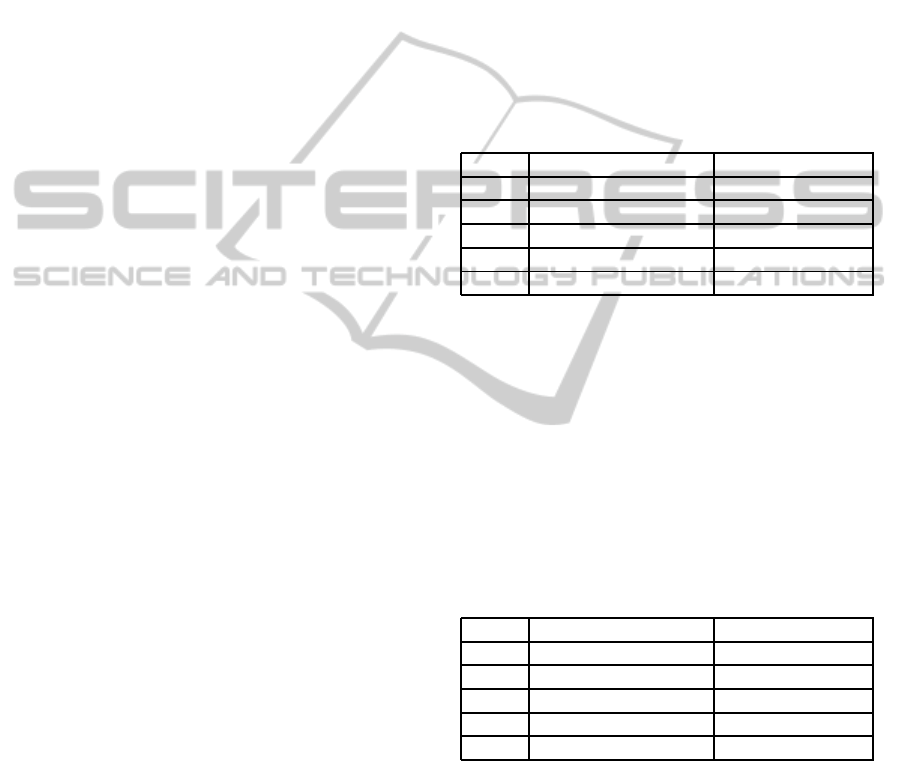
4.8 On DDSM Dataset Classification
We show now the results obtained on DDSM dataset.
In this comparison, we use the same classifiers used
in the previous classification. Also in this case we test
the descriptors of Haralick (HA), Tamura (TA), Bat-
tiato (BA), Haralick-Tamura (HT), Haralick-Battiato
(HB), Tamura-Battiato (TB) and Haralick-Tamura-
Battiato (HTB). The results are resumed in Table 10
and Table 11. Also in this comparison, in fact, as it
can be seen from the tables, the descriptors individu-
ally considered lead to a low accuracy level, while the
percentage of instances correctly classified increases
with the combination in pairs until reaching the max-
imum value when these three basic descriptors are
used all together. In conclusions, the second exper-
iment has confirmed the previous results.
5 CONCLUSIONS
The purpose of this work was to study which com-
bination among the simple descriptors proposed by
Tamura (Tamura et al., 1978), Battiato(Battiato et al.,
2003) and Haralick(Haralick, 1979) leads to a bet-
ter classification of images containing different tex-
Table 10: Results by using DDSM dataset without feature
selection.
NB RBF KNN R-F R-T
HA 49.1% 46.7% 49% 52.4% 48.8%
TA 48.7% 52.1% 48.7% 47.5% 47.1%
BA 44.9% 45.3% 39.4% 37.2% 40.3%
HT 55.3% 54% 56.6% 51.7% 59.6%
HB 56.4% 56% 56.4% 54.5% 49.4%
TB 59.1% 58.4% 62.2% 50.5% 42.5%
HTB 60.5% 60.2% 63.2% 62.1% 48.3%
Table 11: Results by using DDSM dataset with feature se-
lection.
NB RBF KNN R-F R-T
HA 49.1% 48.6% 49.6% 53.1% 51.7%
TA 52.6% 52.6% 48.7% 47.5% 47.1%
BA 48.1% 46% 46.3% 48.8% 51.4%
HT 65.8% 64% 66.5% 60.4% 60%
HB 62.8% 63.1% 64.2% 61.3% 46.1%
TB 64% 65.2% 66.7% 64.4% 62.6%
HTB 66.9% 68.1% 70% 68.1% 49.5%
ture. At the beginning, we tested the individual de-
scriptors discussed above, obtaining an average accu-
racy value of about 74.5% by using Tamura’s features,
77.8% by using Battiato’s features and 78.2% by us-
ing Haralick’s features (on Brodatz album). Already
in this case, the accuracy value is high but we have de-
cided to combine the descriptors to improve the per-
centage of instances correctly classfied. So we have
combined in pairs these descriptors getting an average
of accuracy of about 95.3% by using Battiato’s and
Tamura’s features, 89.7% by using Battiato’s and Har-
alick’s features, 93.6% by using Tamura’s and Haral-
ick’s features. Combining in pairs these descriptors
we have a very high accuracy level. Finally, using
all descriptors, we have an average of accuracy value
about of 94.8%. The efficacy of the three basic de-
scriptors combination is confirmed by the second ex-
periment, even the accuracy level is not excellent but
encouraging. In conclusions, since their easy and fast
calculation, our future interest of course will be a pos-
sible integration of them with equally simple descrip-
tors in a system for image retrieval, in particular for
biomedical imaging where texture can be used to dis-
criminate between healthy and diseased tissue.
ACKNOWLEDGEMENTS
This work has been funded by Regione Autonoma
della Sardegna (R.A.S.) Project CRP-17615 DENIS:
Dataspace Enhancing Next Internet in Sardinia.
VISAPP2014-InternationalConferenceonComputerVisionTheoryandApplications
616

REFERENCES
Battiato, S., Gallo, G., and Nicotra, S. (2003). Perceptive
visual texture classification and retrieval. In Image
Analysis and Processing, 2003.Proceedings. 12th In-
ternational Conference on, pages 524–529.
Brodatz, P. (1966). Textures, a photographic album for
artists and designers. New York:Dover.
Broek, E. and Rikxoort, E. (2005). Parallel-sequential tex-
ture analysis. In Pattern Recognition and Image Anal-
ysis, volume 3687 of Lecture Notes in Computer Sci-
ence, pages 532–541. Springer Berlin Heidelberg.
Chang, C.-Y. and Fu, S.-Y. (2006). Image classification us-
ing a module rbf neural network. In Innovative Com-
puting, Information and Control, 2006. ICICIC ’06.
First International Conference on, volume 2, pages
270–273.
Deselaers, T., Keysers, D., and Ney, H. (2004). Features
for image retrieval - a quantitative comparison. In In
DAGM 2004, Pattern Recognition, 26th DAGM Sym-
posium, pages 228–236.
Haralick, R. (1979). Statistical and structural approaches to
texture. Proceedings of the IEEE.
Hayes K.C., Shah A.N., R. A. (1974). Texture coarseness:
Further experiments. Systems, Man and Cybernetics,
IEEE Transactions on, SMC-4(5):467–472.
Heath, M., Bowyer, K., Kopans, D., Kegelmeyer, P.,
J., Moore, R., Chang, K., and Munishkumaran, S.
(1998). Current status of the digital database for
screening mammography. In Karssemeijer, N., Thi-
jssen, M., Hendriks, J., and Erning, L., editors, Digital
Mammography, volume 13 of Computational Imaging
and Vision, pages 457–460. Springer Netherlands.
Howarth, P. and Rger, S. (2004). S.: Evaluation of tex-
ture features for content-based image retrieval. In In:
Proceedings of the International Conference on Image
and Video Retrieval, Springer-Verlag.
Jian, M., Liu, L., and Guo, F. (2009). Texture image clas-
sification using perceptual texture features and gabor
wavelet features. In Information Processing, 2009.
APCIP 2009. Asia-Pacific Conference on, volume 2,
pages 55–58.
Julesz, B. (1981). Textons, the elements of texture percep-
tion, and their interactions. Nature, 290(5802):91–97.
Landy, M. S. and Graham, N. (2004). Visual perception of
texture. In THE VISUAL NEUROSCIENCES, pages
1106–1118. MIT Press.
Prasad, B. G. and Krishna, A. N. (2011). Statistical texture
feature-based retrieval and performance evaluation of
ct brain images. In Electronics Computer Technology
(ICECT), 2011 3rd International Conference on, vol-
ume 2, pages 289–293.
Rosenfeld, A. (1975). Visual texture analysis: An overview.
Technical report, DTIC Document.
Tamura, H., Mori, S., and Yamawaki, T. (1978). Textu-
ral features corresponding to visual perception. Sys-
tems, Man and Cybernetics, IEEE Transactions on,
8(6):460–473.
Umarani, C. and Radhakrishnan, S. (2007). Combined sta-
tistical and structural approach for unsupervised tex-
ture classification. ICGST International Journal on
Graphics, Vision and Image Processing, 07:31–36.
van den Broek, E. L. and Rikxoort, E. M. (2004). Evalu-
ation of color representation for texture analisys. In
Verbrugge, R., Taatgen, N., and Schomaker, L., ed-
itors, Prooceedings of the 16th Belgian Dutch Artifi-
cial Intelligence Conference (BNAIC 2004), Gronin-
gen, The Netherlands, pages 35–42.
van den Broek, E. L., Rikxoort, E. M., Kok, T., and Schuten,
T. E. (2006). M-hints: Mimicking humans in texture
sorting. In Human Vision and Electronic Imaging XI,
volume 6057, pages 332–343. SPIE, the International
Society for Optical Engineering.
van Rikxoort, E. M., van den Broek, E. L., and Schouten,
T. E. (2005). Mimicking human texture classification.
In Proceedings of Human Vision and Electronic Imag-
ing X, pages 215–226.
StatisticalFeaturesforImageRetrieval-AQuantitativeComparison
617
