
Detecting Events in Crowded Scenes using Tracklet Plots
Pau Climent-P
´
erez
1
, Alexandre Mauduit
2
, Dorothy N. Monekosso
3
and Paolo Remagnino
1
1
Robot Vision Team (RoViT), Kingston University, Penrhyn Road Campus,
KT1 2EE, Kingston upon Thames, U.K.
2
Department of Computing,
´
Ecole Nationale Sup
´
erieure d’Ing
´
enieurs de Caen (ENSICAEN), Caen, France
3
Engineering Design and Mathematics, University of the West of England, Bristol, U.K.
Keywords:
Tracklet Exploitation, Tracklet Plot, Bag-of-Words, Kmeans, Video Analytics, Crowd Analytics, Video
Surveillance.
Abstract:
The main contribution of this paper is a compact representation of the ‘short tracks’ or tracklets present in a
time window of a given video input, which allows to analyse and detect different crowd events. To proceed,
first, tracklets are extracted from a time window using a particle filter multi-target tracker. After noise removal,
the tracklets are plotted into a square image by normalising their lengths to the size of the image. Different
histograms are then applied to this compact representation. Thus, different events in a crowd are detected via
a Bag-of-words modelling. Novel video sequences, can then be analysed to detect whether an abnormal or
chaotic situation is present. The whole algorithm is tested with our own dataset, also introduced in the paper.
1 INTRODUCTION
Automatic analysis of crowded scenes appears as a
need to reduce costs and improve people’s safety,
while reducing the burden of manual video surveil-
lance (Candamo et al., 2010; Davies et al., 1995).
Crowd analysis has received attention in the last
decade, and is of interest for a very wide range of
fields, as described in (Zhan et al., 2008; Jacques Ju-
nior et al., 2010).
There are different ways to approach crowd dy-
namics modelling. Many different scenes, ranging
from sparse scenes, with few individuals, to crowds,
all forming a continuum. This calls for a topology
of scenes, such as the one proposed by (Zhan et al.,
2008), with three levels: micro-, meso- and macro-
scopic which would be roughly equivalent to indi-
vidual, group or crowd levels. Topologies show the
human need for categorisation of situations, but this
does not mean that interaction among methods from
different levels cannot be possible.
In fact, in Thida et al. (Thida et al., 2013), the au-
thors state that approaches considered to be part of the
microscopic modelling (as it is the tracking of individ-
uals in a scene) can be used in a bottom-up approach,
which allows us to look at crowded situations from
the individual tracking perspective.
In this paper, we will present an idea based on
that concept. To do this, we obtain short tracks from
the people in the scene, and then use this informa-
tion and merge it into the ‘tracklet plot’, a feature
that will be described in Subsection 2.2. After that,
a bag of words modelling will extract the most com-
mon words, and their appearance frequencies in dif-
ferent situations (Section 2.3). We will also introduce
a novel dataset for crowded scene analysis from mul-
tiple views. Finally, the results for our method, as
well as the conclusions drawn will be presented in
Section 4.
1.1 Event Recognition and Tracklet
Exploitation
The work by Ballan et al. (Ballan et al., 2011) surveys
the field of event recognition, from interest point de-
tectors and descriptors, to event modelling techniques
and knowledge management technologies. The au-
thors imply that the recognition of crowd events, and
the recognition of actions, performed by a single actor
using a single camera, have much in common, since
the event modelling techniques can be quite similar,
if not the same, regardless of the feature being used,
which will depend on the case.
Hu et al. (Hu et al., 2008) are able to extract
the dominant motion patterns of a video, by using
sparse optical flow vectors as their tracklets, these
are then associated into motion patterns by a sink-
174
Climent-Pérez P., Mauduit A., N. Monekosso D. and Remagnino P..
Detecting Events in Crowded Scenes using Tracklet Plots.
DOI: 10.5220/0004742301740181
In Proceedings of the 9th International Conference on Computer Vision Theory and Applications (VISAPP-2014), pages 174-181
ISBN: 978-989-758-004-8
Copyright
c
2014 SCITEPRESS (Science and Technology Publications, Lda.)

seeking process, followed by the construction of super
tracks which represent the dominant/collective mo-
tion patterns discovered. The authors obtain the dom-
inant motion patterns or trajectories, and these can be
used to detect deviations from the pattern. Neverthe-
less, other types of events cannot be detected. Las-
das et al. (Lasdas et al., 2012) use tracklets obtained
from a Kanade-Lucas-Tomasi (KLT) tracker, instead
of sparse flow vectors. Furthermore, they enumerate
the desirable features of a motion summarisation sys-
tem to which the reader is referred.
Similarly, in G
´
arate et al. (Garate et al., 2009), the
authors track FAST points (Features from Accelerated
Segment Test) extracted from the bounding boxes of
objects detected via background subtraction. Density
is estimated in the image by superimposing a grid and
counting the number of FAST feature points in each
cell in the grid. Furthermore, the tracklets extracted
from the tracking of the FAST features are used to
detect dominant directions of motion.
On the other hand, Dee and Caplier (Dee and
Caplier, 2010) present an analysis of crowd events
based on histograms of motion direction (HMDs),
which, to some extent are similar to the tracklet plot,
except for the fact that the HMDs are obtained for
the whole video sequence, instead of smaller inter-
vals, as is done in this paper. Using small intervals al-
lows the analysis of particular situations happening at
a given moment in a long video, rather than analysing
the video as a whole.
2 METHODOLOGY
There are two main contributions in this paper. On the
one hand, a feature based on the compact representa-
tion of tracklets is presented (see Fig. 2 for examples).
On the other, a dataset for crowded scene analysis is
introduced. In this section, the first contribution will
be explained.
The proposed feature enables the detection of
anomalous events in crowded scenarios. The tracklet
plot representation is, to some extent, similar to the
Motion History Images (MHI) introduced by Bobick
and Davis (Bobick and Davis, 2001), but instead, the
tracklet superimposition represents the density and or-
derliness of a particular interval: for instance, if all the
tracklets are parallel they will generate an area in the
image that is particularly bright (high intensity in a
narrow band), while a chaotic situation will be repre-
sented by an image which has no particular bright ar-
eas. Figure 1 shows an overview of the whole feature
extraction process, including also the training stage.
Video interval
of Δ frames
Inial boun-
ding boxes
Tracklets for
interval (TS)
Filtered
tracklets (FTS)
Tracklet plot
Histogram for
interval (h
s,int
)
Video se-
quence (S)
Bag-of-words training
h
s,1
h
s,2
h
s,3
h
s,4
h
s,5
...
w
1
w
1
w
2
w
2
w
1
...
Tracking
Noise
removal
Plong
Histogram
W
s
H
s
η
s
w1 w2 w3
Figure 1: Overview of the whole process up to Bag-of-
words training.
2.1 Tracking Multiple Targets
The first step of the algorithm entails the extraction
of short tracks or tracklets. To do this, a tracking al-
gorithm needs to be employed. Most trackers need
an initialisation step, in which the moving objects or
people are detected. Once the algorithm has its ini-
tialisation seeds, the tracking then proceeds automat-
ically.
Furthermore, in our case, multiple targets need to
be tracked at the same time, in order to obtain the mo-
tion patterns of the whole scene. Thus, a multi-target
tracker, or a tracker running in parallel for each de-
tected individual must be used. In this step, a Particle
Filter based algorithm is used (P
´
erez et al., 2002), and
run in parallel for each of the individuals present in
the scene.
2.1.1 Tracklet Extraction
Since most trackers deal badly with tracking over long
periods of time, intervals of ∆ frames are used. Track-
let sets T S
n∆
are obtained for each interval, where
n is the interval number and so n · ∆ is the initial
frame for that tracklet set. These sets will contain
the tracklets for each individual being tracked dur-
ing the interval. At this point, the tracklet sets con-
sist of a series of 2D points for each individual; so
T S = {P
t=0
, ··· , P
∆−1
}, that is, for each frame t, P is
a set of 2D points, containing the centres of mass of
the bounding boxes of the people being tracked. It has
the form: P
t
= {c
0
, · ·· , c
M
}, where each c
i
represents
the center of mass of a tracked box with id i, and M
is the total amount of individuals in the scene for the
tracklet set T S.
Since the Particle Filter tracker yields a noisy out-
put due to the change in scale of the bounding boxes
that happens during tracking, a Kalman filter is ap-
plied to the sequences of centres of mass, so that
DetectingEventsinCrowdedScenesusingTrackletPlots
175

smoother tracklets are retrieved. By doing so, a se-
ries of filtered tracklet sets FT S are obtained.
2.2 Feature Extraction
Feature extraction is performed in two steps. The first
step consists of tracklet plotting. This step plots the
tracklets into a fixed-size image, centered and nor-
malised (Sec. 2.2.1). Then, in the second step, a his-
togram is obtained from the image, which allows fur-
ther analysis of the individuals’ speed and direction
of motion (Sec. 2.2.2).
2.2.1 Tracklet Plotting
Once the tracklets have been filtered, the compact rep-
resentation is obtained, namely the tracklet plot. To
do so, the tracklets in each set FT S are first fit into a
square image by normalising their lengths to the size
of the image. Each filtered tracklet f t in the set is
assigned an equal weight:
weight =
I(max)
||FT S||
(1)
which is represented as an intensity value in the im-
age. Here, I(max) is the maximum intensity (255 for
8-bit images) and ||·|| denotes the number of elements
in the filtered tracklet set FT S. Each tracklet is then
centered and superimposed in the tracklet plot, as it
is depicted in Fig. 2. It is worth noting that this rep-
resentation tracks global behaviour, and not situated
actions.
(a)
(b)
(c)
(d)
1
2
Figure 2: Example of different tracklet plots. a) Ordered
group of people walking at the same speed and direction; b)
a fast biker (b.2) and a slower pedestrian (b.1); c) Two peo-
ple walking in perpendicular directions; d) A chaotic situa-
tion, where people run away. Pictures are shown in inverted
colour and enhanced contrast.
2.2.2 Histogram Extraction
After the above process, a histogram can be extracted
from the tracklet plot. To do this, two methods are
proposed:
• Circular Histogram. This histogram takes con-
centric disc-shaped regions R into account, be-
ing R = r
0,ρ−1
, r
ρ,2ρ−1
, · ·· , r
nρ,max
a set of ranges,
where r
0,ρ
is a circular region around the centre of
the image with a radius of ρ, and max is the radius
of the image. The histogram for a given window
(of a sequence s) h
(s,win)
is then calculated as:
h
(s,win)
(r, I(x)) =
∑
p
i
∈r
I(p
i
) if I(p
i
) = I(x), ∀r ∈ R,
(2)
where each p
i
is a pixel in the region r. The
main advantage of this kind of histogram is that
it can control differences in velocity for the differ-
ent tracked individuals.
• Angle-distance Histogram. On the other hand,
a histogram based on sectors can be better to de-
tect the orderliness of a crowd, since it can de-
tect whether all the tracklets follow a particu-
lar direction of motion, or an small amount of
them, or the movement in the scene is chaotic,
with individuals running in many different direc-
tions. For this, sectors A are introduced, such that
A = α
0,γ−1
, · ·· , α
(n−1)γ,nγ
being γ the angle span
for each sector and with nγ = 2π. Thus, the equa-
tion for the histogram can be modified from (2),
to look like:
h
(s,win)
(α, r, I(x)) =
∑
p
i
∈(r,α)
I(p
i
) | I(p
i
) = I(x), (3)
for all r ∈ R and all α ∈ A.
Furthermore, two more histogram extraction
methods have been envisaged, each one based on the
two already presented, but with the particularity that
they have one fewer dimension (totalling 1 dimension
for the circular counterpart, and 2 dimensions for the
angle-distance). In these two modalities, the binning
in the intensity dimension is not performed; instead,
only the count of pixels in the plot that are not equal to
zero is kept. Different experiments have been carried
out, in order to establish which is the best histogram
modality to use (see Sec. 3).
Regardless of the method employed, all the his-
tograms h
(s,win)
are normalised to sum 1. Since the
method is applied to each window of a video se-
quence, sets of histograms H
s
can be obtained for each
sequence s in the set of video sequences for training.
Figure 3 shows the two main histogram modalities for
clarity; a) shows the circular histogram, with the dif-
ferent regions with their radius being multiples of ρ.
max depicts the maximum plot radius. In the same fig-
ure, in b) the γ angle span is also shown, along with
the lines delimiting the sectors.
2.3 Bag of Words Modelling
To perform a modelling of the different crowd situa-
tions in the video input, a series of training video se-
quences S
train
are employed. Each sequence s has an
VISAPP2014-InternationalConferenceonComputerVisionTheoryandApplications
176

max
ρ
max
ρ
γ
(a)
(b)
Figure 3: Example of the two main histogram extraction
modalities presented: a) circular histogram; b) polar his-
togram.
associated set of histograms H
s
. And h
(s,win)
denotes
the histogram for an interval (win) of sequence s.
A bag-of-words (BoW) modelling is applied to
the sequences (Sivic and Zisserman, 2003). This ap-
proach was first used for the categorisation of docu-
ments in a corpus, and introduced the concept of a his-
togram of key word frequencies (Ballan et al., 2011).
In our case, a video is the analogue of a document;
the words in our documents will be tracklet plot his-
tograms; and the “key words” frequency histograms
for each document will be extracted by the BoW al-
gorithm as follows:
• Step 1. First, all the sequences of tracklet plot his-
tograms (H
s
) are taken, and the tracklet plot his-
tograms (h
(s,win)
) are fed into a k-Means cluster-
ing, regardless of the sequence they are originally
part of. This will return a fixed number of cluster
representatives or key words (w).
• Step 2. These key words are used to generate key-
word sequences (W
s
), in which each of the original
words is replaced by the nearest key word from
Step 1.
– The distance to the a key word w is calculated
by the Jeffrey distance, as:
J(h
(s,win)
, w) =
KL(h
(s,win)
, w) + KL(w, h
(s,win)
)
2
,
(4)
where KL(·, ·) is the Kullback-Leibler distance
between the key word, or more generally for
two discrete probability distributions p, q:
KL(p, q) =
||p||
∑
i=1
p
i
ln
p
i
q
i
, (5)
for all p
i
, q
i
| p
i
6= 0 and q
i
6= 0.
• Step 3. A histogram of key-word frequencies (η)
is obtained for each key-word sequence W
s
. Each
bin of this histogram is:
η
s
(w) =
||W
s
||
∑
x=1
δ(w, W
s
(x)), (6)
being
δ(w, W
s
(x)) =
1 if W
s
(x) = w,
0 otherwise.
(7)
• Step 4. All η
s
histograms are then normalised to
sum 1, this will make them invariant to sequence
length.
Once this process is finished, the model is trained,
and any future video input can be recognised by
means of the k-nearest neighbour (k-NN) algorithm.
3 EXPERIMENTATION
The algorithm described in the previous subsection
(Sec. 2.3), has been used to evaluate the performance
of the feature described in subsection 2.2. To do
so, first a dataset was acquired. Then, a valida-
tion was performed, using a leave-one-sequence-out
cross-validation (LOOCV). In the next subsections,
the set-up is explained in more detail.
3.1 The Penrhyn Road Campus Dataset
A set of four cameras were placed in a building
adjoining the courtyard in the Penrhyn Road cam-
pus. Two cameras were installed on the second floor,
and two were placed on the fourth floor, all over-
looking the courtyard. A group of 20 actors per-
formed various stage group behaviours in the court-
yard, such as walking normally as one group, walking
normally as two crossing groups, walking in one di-
rection with some people abnormally deviating from
the trajectory followed by the rest, or simulating a
chaotic event where everybody runs away from a dan-
ger. These videos have been labelled into three cate-
gories, namely normal, abnormal and chaotic, re-
spectively. For the purpose of this work, 18 sequences
from one of the views are used. Table 1 summarises
the details of the dataset.
Table 1: Characteristics of the dataset.
Category Sequences
Normal 10
Abnormal 5
Chaotic 3
DetectingEventsinCrowdedScenesusingTrackletPlots
177

Figure 4: Example of a frame from a chaotic (panic event)
situation from the Penrhyn Road Courtyard dataset.
3.2 Testing Set-up and Validation
To test our method, a set of features (H) needs to be
obtained. It is a superset formed by all the sets of fea-
tures H
s
| s ∈ S, which in turn contain all the features
for all the intervals of sequence s: h
(s,win)
. The bag
of words modelling algorithm takes H as input and
yields a set of key-words w and the set of key-word
frequency histograms η (one per sequence: η
s
).
In order to validate our method, a leave-
one-sequence-out cross-validation (LOOCV) is em-
ployed. This process will take all the sequences ex-
cept for one, and create the training sequences set
S
train
= S −s
test
. Then H
train
is obtained as per the pro-
cess already described; subsequently, the BoW model
is trained. Then, the test sequence, s
test
is used to
check. This is done for all the folds, that is, by leaving
one sequence out for test at each fold.
All the steps through the process involve a num-
ber of parameter decisions, set as shown in Table 2.
The parameter iter is in reference to the number of
iterations that the k-Means algorithm is run during
the Bag-of-words model acquisition. The parameter
named reps is the number of times that the BoW is
run per test. Also, Table 3 is given, which shows the
bins used for the different histogram extraction meth-
ods employed.
Table 2: Parameters used for the validation of the method.
Parameter Value or range
∆ 50
plot radius 50
h
(s,win)
bins See Table 3
k-Means K 2–64
k-Means iter 1; 3
BoW reps 5; 15
Table 3: Size (as number of bins) for the histograms used.
Histogram Bins
Circular 6 × 255
Polar 8 × 6 × 255
Circular w/o int. 10
Polar w/o int. 8 × 6
4 RESULTS AND CONCLUSIONS
As said, different configurations have been tested. Ta-
ble 2 shows the values which have been used for each
of the parameters. These have been obtained experi-
mentally.
The k-Means clustering algorithm is prone to give
different results due to the random process related to
the cluster centre selection. As said, the variable iter
is related to the number of times the k-Means is run.
The clustering error is calculated each time, and the
clustering with the lower error is picked at the end
of the process. On the other hand, the Bag-of-Words
modelling can also be run multiple times (repetitions
or reps) with different k-Means centres, so that the
random initialisation problem is overcome.
Two different configurations have been tried, once
with iter = 3 and reps = 5; as well as iter = 1, and
reps = 15. Table 3 shows the size of the histograms
that have been used for the different modalities.
Figure 5 shows the results in a graphical form,
each of the series representing a different configura-
tion. Four series are shown in the figure. CI stands
for circular histogam, and LP stands for polar. Both
include intensity bins. The numbers next to the two
letters (CI or LP) correspond to the iterations of k-
Means (iter) and the repetitions of BoW (reps), re-
spectively.
Figures 6 and 7 show the behaviour of the algo-
rithm for the polar histogram that has been presented,
both without and with intensity bins respectively. It
is worth noting that the best result is achieved when
no intensity bins are used and reaches a maximum
success rate of 83% (K = 2). In the case of using
intensity bins, the maximum success rate is of 67%
(K = 2). Table 4 shows the maximum, mean and min-
imum success rates for the both modalities of polar
histogram.
Figures 8 and 9 show the behaviour of the algo-
rithm for the circular histogram that has been pre-
sented, both without and with intensity bins respec-
tively. In this case, the maximum success rates are
72.7% (K = 21), for the circular histogram without
intensity bins; and 61.6% (K = 7) for the histogram
with intensity bins. Table 5 shows the maximum,
VISAPP2014-InternationalConferenceonComputerVisionTheoryandApplications
178
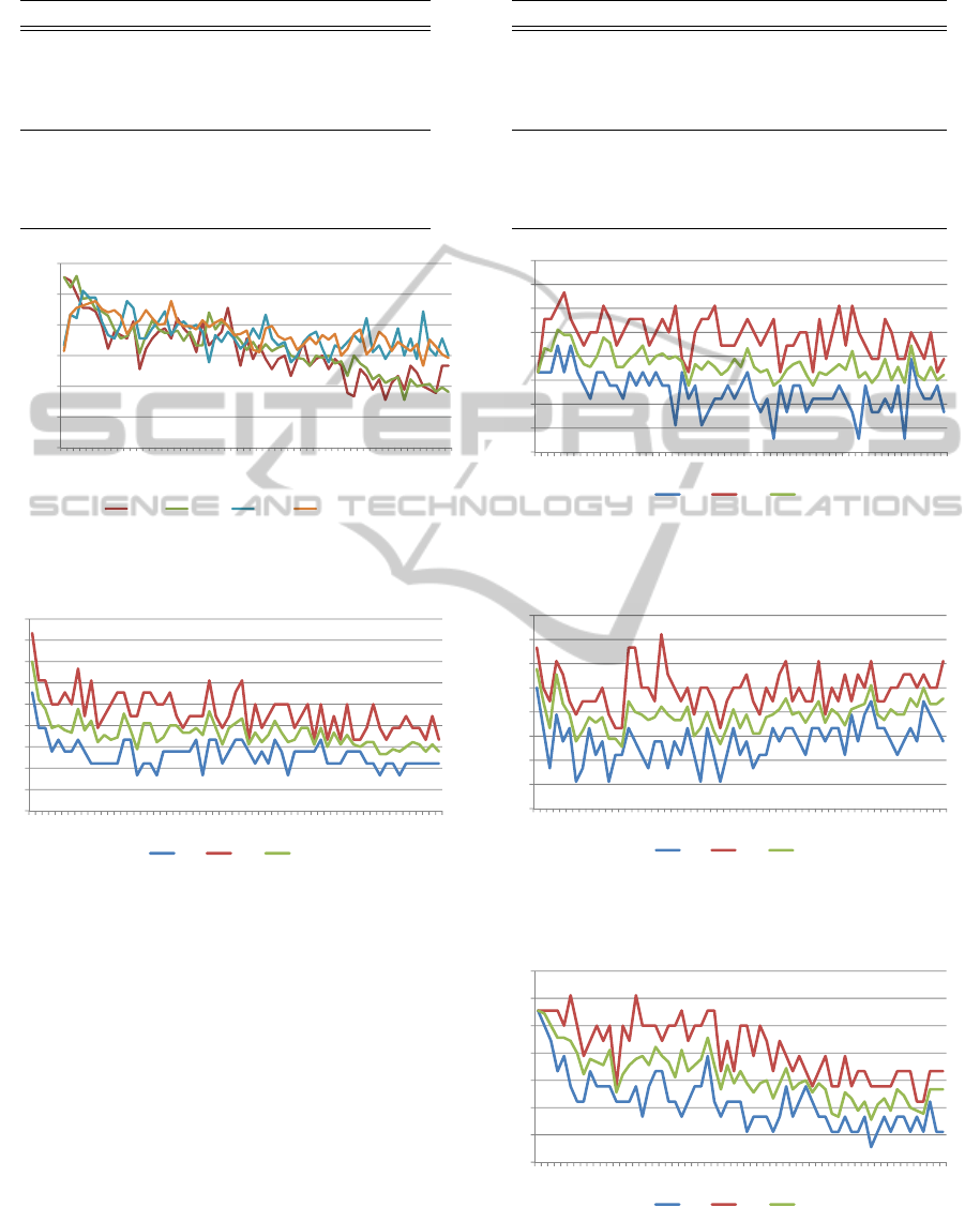
Table 4: Results for polar histograms.
Histogram Success % K
Polar
Lowest Min. 5.6% K = 51
Highest Max. 66.7% K = 6
Highest Mean. 51.5% K = 5
Polar w/o intensities
Lowest Min. 16.7% K = 18
Highest Max. 83.3% K = 2
Highest Mean. 70.0% K = 2
0,00%
10,00%
20,00%
30,00%
40,00%
50,00%
60,00%
2 4 6 8 10 12 14 16 18 20 22 24 26 28 30 32 34 36 38 40 42 44 46 48 50 52 54 56 58 60 62
Success rate (%)
Number of words (K)
CI 3,5 CI 1,15 LP 3,5 LP 1,15
Figure 5: Graphical view of the success rate for increas-
ing values of K, using polar and circular histograms (with
intensity bins).
0
10
20
30
40
50
60
70
80
90
2 8 14 20 26 32 38 44 50 56 62
min max avg
Figure 6: Maximum, mean and minimum success rates for
increasing values of K using the polar histogram (without
intensity values).
mean and minimum success rates for the both modal-
ities of circular histogram.
4.1 Discussion and Conclusions
A compact representation of the tracklets present in
a time window of a given video input has been pre-
sented. Tracklets are extracted from a time window
using a particle filter multi-target tracker. Noise is
then filtered out, to obtain smooth tracklet trajecto-
ries. The tracklets are then plotted into a square
image, and a circular histogram is then applied to
this compact representation. Furthermore, a Bag-of-
words modelling has been employed over these fea-
Table 5: Results for circular histograms.
Histogram Success % K
Circular
Lowest Min. 5.6% K = 53
Highest Max. 61.6% K = 7
Highest Mean. 55.6% K = 2
Circular w/o intensities
Lowest Min. 11.1% K = 8
Highest Max. 72.2% K = 21
Highest Mean. 57.8% K = 2
0
10
20
30
40
50
60
70
80
2 8 14 20 26 32 38 44 50 56 62
min max avg
Figure 7: Maximum, mean and minimum success rates for
increasing values of K using the polar histogram (with in-
tensity values).
0
10
20
30
40
50
60
70
80
2 8 14 20 26 32 38 44 50 56 62
min max avg
Figure 8: Maximum, mean and minimum success rates for
increasing values of K using the circular histogram (without
intensity values).
0
10
20
30
40
50
60
70
2 8 14 20 26 32 38 44 50 56 62
min max avg
Figure 9: Maximum, mean and minimum success rates for
increasing values of K using the circular histogram (with
intensity values).
DetectingEventsinCrowdedScenesusingTrackletPlots
179

tures for crowd event recognition. Our method has
been validated by using a LOOCV cross-validation
on a novel dataset.
From the results, some conclusions can be drawn.
First, it can be seen that results are generally better
for lower values of K. This seems to be logical, since
there should be, at most, three or four different situa-
tions at a given moment in time; that is: normal, devi-
ations from normal and chaotic. Also, it can be seen
that results with histograms that do not take inten-
sity into account are better than their intensity-aware
counterparts. Finally, polar histogram seems to per-
form better than circular; which again, seems logical
due to the fact that the circular histogram does not
take orderliness into account.
It has to be noted that the dataset in use in this case
is a very challenging one, due to the presence of heavy
clutter due to objects in the scene (trees, benches...)
which complicates the tracking, which is the bottle-
neck of the process. A poor tracking result will al-
ways yield to worse results in general. Further work
needs to be carried out in this regard.
4.2 Future Work
In this section a series of immediate and future im-
provements are shown, which are considered to ame-
liorate the results.
As just said, the bottleneck of the whole process is
in the tracking. If the tracking fails, the tracklet plots
will not be representative of the situation in the scene.
For this reason, a good tracker is essential. Track-
ing perfectly and flawlessly is still an open challenge
in the computer vision research community. Thus,
and since the aim of this work is not achieving bet-
ter tracking, ground truth data of the people could be
used to evaluate the tracklet plot histograms and the
bag-of-words modelling being applied. Another op-
tion would be using promising trackers such as the
recent work by Kwon et al. (Kwon and Lee, 2013).
Furthermore, testing our method on other datasets
is a pending task. Nevertheless, most existing datasets
are near-field, and thus, ours seems more appropriate
for group and crowd analysis. Also, most of them pro-
vide video footage from a single view. Furthermore,
the types of situations present in our dataset, are not
always present in other publicly available datasets.
For instance, the UMN dataset
1
, would be the best
candidate to try our algorithm next. However, it has
two main drawbacks: first, it includes scenes were
people wander, which is not considered ‘normal’ be-
haviour as defined and used in this paper; second, it
1
http://mha.cs.umn.edu/proj events.shtml (Accessed:
Nov. 2013)
is single view, so planned extensions of our work for
multiple views could not be tested on it.
Finally, as just mentioned, future work also in-
cludes the use of video footage from multiple views.
To this end, information from all the available cam-
eras (four in our dataset) is to be combined and tested
either by a fusion method at the “feature level”, or
by merging by means of a “model-level” algorithm.
For the former, synchronised video is to be used, so
obtaining the features from the various video sources
simultaneously. The features are then fused by merg-
ing them into a longer feature. Dimensionality reduc-
tion techniques might be needed, since the features
are now much longer (i.e. four-fold) than the origi-
nal. In the latter, on the other hand, different models
for the different cameras are learnt, and then fusion
is performed afterwards, using a voting mechanism,
that in turn could assign weights to the different views
(e.g. by using an additional neural network layer).
ACKNOWLEDGEMENTS
This work has been supported by the European
Commission’s Seventh Framework Programme (FP7-
SEC-2011-1) under grant agreement N.
o
285320
(PROACTIVE project).
REFERENCES
Ballan, L., Bertini, M., Del Bimbo, A., Seidenari, L., and
Serra, G. (2011). Event detection and recognition for
semantic annotation of video. Multimedia Tools and
Applications, 51(1):279–302.
Bobick, A. and Davis, J. (2001). The recognition of human
movement using temporal templates. Pattern Analy-
sis and Machine Intelligence, IEEE Transactions on,
23(3):257–267.
Candamo, J., Shreve, M., Goldgof, D. B., Sapper, D. B.,
and Kasturi, R. (2010). Understanding Transit Scenes:
A Survey on Human Behavior-Recognition Algo-
rithms. IEEE Transactions on Transportation Sys-
tems, 11(1):206–224.
Davies, A., Yin, J., and Velastin, S. (1995). Crowd monitor-
ing using image processing. Electronics & Communi-
cation Engineering Journal, 7(1):34–47.
Dee, H. M. and Caplier, A. (2010). Crowd behaviour anal-
ysis using histograms of motion direction. In Im-
age Processing (ICIP), 2010 17th IEEE International
Conference on, pages 1545–1548. IEEE.
Garate, C., Bilinsky, P., and Bremond, F. (2009). Crowd
event recognition using hog tracker. In Performance
Evaluation of Tracking and Surveillance (PETS-
Winter), 2009 Twelfth IEEE International Workshop
on, pages 1–6.
VISAPP2014-InternationalConferenceonComputerVisionTheoryandApplications
180

Hu, M., Ali, S., and Shah, M. (2008). Detecting global mo-
tion patterns in complex videos. In Pattern Recogni-
tion, 2008. ICPR 2008. 19th International Conference
on, pages 1–5. IEEE.
Jacques Junior, J., Raupp Musse, S., and Jung, C. (2010).
Crowd analysis using computer vision techniques.
Signal Processing Magazine, IEEE, 27(5):66–77.
Kwon, J. and Lee, K. (2013). Wang-Landau Monte Carlo-
based Tracking Methods for Abrupt Motions. Trans-
actions on Pattern Analysis and Machine Intelligence,
35(4):1011–1024.
Lasdas, V., Timofte, R., and Van Gool, L. (2012). Non-
parametric motion-priors for flow understanding. In
Applications of Computer Vision (WACV), 2012 IEEE
Workshop on, pages 417–424. IEEE.
P
´
erez, P., Hue, C., Vermaak, J., and Gangnet, M. (2002).
Color-Based Probabilistic Tracking. In European
Conference on Computer Vision 2002, pages 661–675.
Sivic, J. and Zisserman, A. (2003). Video google: a text
retrieval approach to object matching in videos. In
Computer Vision, 2003. Proceedings. Ninth IEEE In-
ternational Conference on, pages 1470–1477 vol.2.
Thida, M., Yong, Y. L., Climent-P
´
erez, P., How-lung, E.,
and Remagnino, P. (2013). A Literature Review on
Video Analytics of Crowded Scenes. In Cavallaro,
A. and Atrey, P. K., editors, Intelligent Multimedia
Surveillance: Current Trends and Research, pages 1–
23. Springer (in press).
Zhan, B., Monekosso, D. N., Remagnino, P., Velastin, S. A.,
and Xu, L.-Q. (2008). Crowd analysis: a survey. Ma-
chine Vision and Applications, 19(5-6):345–357.
DetectingEventsinCrowdedScenesusingTrackletPlots
181
