Evaluation of Color Spaces for Robust Image Segmentation

Alexander Jungmann, Jan Jatzkowski and Bernd Kleinjohann

Cooperative Computing & Communication Laboratory

University of Paderborn, Fuerstenallee 11, Paderborn, Germany

Keywords:

Image Processing, Color-based Segmentation, Color Spaces, Evaluation of Segmentation Results.

Abstract:

In this paper, we evaluate the robustness of our color-based segmentation approach in combination with dif-

ferent color spaces, namely RGB, L

∗

, HSV, and log-chromaticity (LCCS). For this purpose, we describe

our deterministic segmentation algorithm including its gradually transformation of pixel-precise image data

into a less error-prone and therefore more robust statistical representation in terms of moments. To investigate

the robustness of a speciﬁc segmentation setting, we introduce our evaluation framework that directly works

on the statistical representation. It is based on two different types of robustness measures, namely relative

and absolute robustness. While relative robustness measures stability of segmentation results over time, abso-

lute robustness measures stability regarding varying illumination by comparing results with ground truth data.

The signiﬁcance of these robustness measures is shown by evaluating our segmentation approach with differ-

ent color spaces. For the evaluation process, an artiﬁcial scene was chosen as representative for application

scenarios based on artiﬁcial landmarks.

1 INTRODUCTION

Image segmentation refers to the problem of parti-

tioning a single image into regions of interest (ROI)

and a variety of techniques exists for region-based

segmentation (Freixenet et al., 2002). Each ROI de-

scribes a homogenous region where homogeneity is

measured, e.g., by means of features as color, texture,

or contours (Russell and Norvig, 2010). Which fea-

ture or combination of features is used to measure ho-

mogeneity depends on the goal of a certain computer

vision system, i.e. there is an ambiguous choice. Usu-

ally, a computer vision system includes object detec-

tion and recognition whose results are used for high

level applications. Features chosen for segmentation

depend on object characteristics that are assumed to

distinguish objects from their environment. Examples

from embedded systems domain are, e.g., driver as-

sistance systems for trafﬁc sign recognition in the au-

tomotive domain (Mogelmose et al., 2012), obstacle

detection for behavior in robotics (Blas et al., 2008),

or face recognition in biometrics (Yang et al., 2009).

In this paper, we focus on color-based segmen-

tation for an efﬁcient and robust object detection

within embedded systems. While efﬁciency is re-

lated to the implementation of our segmentation ap-

proach, robustness refers to stable segmentation re-

sults in presence of illumination variations and noise

over time. Since environmental illumination inﬂu-

ences color perception, an evaluation of different

color spaces seems promising to achieve robustness.

Various color spaces exist, each aiming at provid-

ing special characteristics, e.g., regarding color dis-

tance, color description, or color ordering. While

some color spaces are based on the assumption

that each color is composed of three primary colors

(trichromatic theory; e.g. RGB, XYZ), other color

spaces aim at adapting human color perception (e.g.

HSV). Since color-based segmentation utilizes color

distances to measure homogeneity of image parti-

tions, the choice of color space has heavy impact on

segmentation results (Busin et al., 2009).

In this paper, we propose an efﬁcient, color-based

segmentation approach. Furthermore, we present an

evaluation of this approach considering varying il-

lumination and different color spaces, namely RGB,

∗

, HSV, and LCCS. The goal of this evalua-

tion is to identify color spaces that provide robust re-

sults with our segmentation approach. Due to the ill-

posed nature of the segmentation problem, evaluation

of segmentation results is a hard challenge (Unnikr-

ishnan et al., 2007). On the one hand, results of an

entire vision system including segmentation typically

contain effects of post-processing steps and there-

fore do not allow to identify segmentation effects.

On the other hand, comparing segmentation results

648

Jungmann A., Jatzkowski J. and Kleinjohann B..

Evaluation of Color Spaces for Robust Image Segmentation.

DOI: 10.5220/0004743406480655

In Proceedings of the 9th International Conference on Computer Vision Theory and Applications (VISAPP-2014), pages 648-655

ISBN: 978-989-758-003-1

 2014 SCITEPRESS (Science and Technology Publications, Lda.)

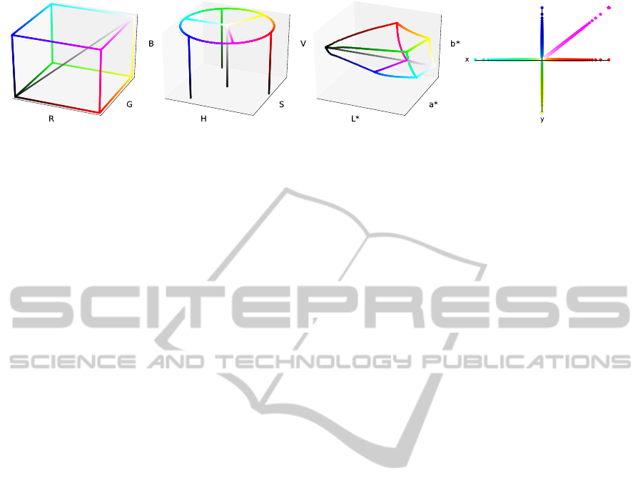
(a) RGB cube edges. (b) HSV color space. (c) L

∗

color space. (d) Log-chromaticity color space.

Figure 1: Visualization of colors from RGB cube edges within considered color spaces.

with ground truth data raises the question: What is

a ground truth segmentation? Considering these chal-

lenges of evaluating segmentation results, we propose

a relative and an absolute robustness measure within

our evaluation framework. By means of these values,

we aim at measuring robustness of segmentation re-

sults within a still scene sequence. In this context, ro-

bustness refers not only to constant regions over time

but also to constant regions at different illumination.

2 COLOR SPACES

Color spaces allow to describe a particular color by

means of basic components. The variety of color

spaces results from differences within these basic

components and many color spaces result from each

other by transformation. Hence, different color spaces

do not have to vary in their covered colors, but rather

differ in the order and scaling of colors. Depending

on the color space, this results in different distances

and distance relations between colors and therefore

effects color-based segmentation (cf. Section 5.1).

In this paper, we consider representatives of pri-

mary, luminance-chrominance, and perceptual color

space classes introduced in (Vandenbroucke et al.,

2003) as well as a variant of log-chromaticity color

space (LCCS) presented in (Finlayson et al., 2009).

RGB and XYZ are well known representatives of

primary color spaces. Since XYZ results from a lin-

ear transformation of RGB and RGB is most widely

used in color image segmentation (Busin et al., 2009),

we consider RGB. In RGB, color is described by its

percentage of the primary colors red, green, and blue.

Due to equidistant scaling of all three primary colors,

RGB color space describes a cube where the main di-

agonal represents gray values (Figure 1(a)).

The perceptual color space HSV describes a color

in cylinder coordinates by its hue, saturation, and a

luminance-inspired value (Szeliski, 2011). Hue is

described by the angle around the vertical axis with

complementary colors 180

◦

opposite one another; sat-

uration and value are usually ranged in [0,1] where

saturation S = 0 corresponds to shades of gray (Fig-

ure 1(b)). In fact, HSV and RGB are related to each

other by a non-linear transformation.

The luminance-chrominance color space L

∗

(also called CIELAB) was originally constructed by

International Commission on Illumination (CIE) with

a non-linear remapping of the primary XYZ color

space to describe differences of colors w.r.t. lumi-

nance and chrominance more perceptually uniform

(Szeliski, 2011). While a

∗

describes green and red

percentage of a color and b

∗

describes its blue and

yellow percentage, L

∗

represents luminance. Hence,

∗

-axis represents all levels of gray (Figure 1(c)).

Furthermore, we consider LCCS which results

from a logarithmic scaled projection of RGB color

space. In (Finlayson et al., 2009), LCCS is derived

based on assumptions of Lambertian reﬂectance,

Planckian lighting, and fairly narrow-band cam-

era sensors. In our evaluation we compute log-

chromaticity colors according to (Khanal et al., 2012):

(x,y) = (log (R/G),log(B/G)). (1)

Figure 1(d) shows a visualization of RGB cube edges

transformed to LCCS by Equation 1. Since projection

effects that one LCCS color represents various RGB

colors, e.g., the point of origin represents all gray val-

ues, this visualization is ambiguous.

3 IMAGE SEGMENTATION

The basic idea of image segmentation is to identify

contiguous blocks of pixels that are homogeneous

with respect to a pre-deﬁned criterion. In our work,

we incorporate color as criterion of homogeneity.

3.1 Segmentation Algorithm

Our deterministic segmentation algorithm processes

an entire image row by row, starting at the topmost

row, at the leftmost pixel within each row. Contigu-

ous blocks of pixels with similar color are identiﬁed

and immediately extracted from the image. The algo-

rithm incorporates two major concepts. (1) Within a

EvaluationofColorSpacesforRobustImageSegmentation

649

(a) (b) (c) (d)

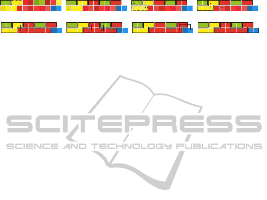
(e) (f) (g) (h)

Figure 2: Segmentation example with exemplary intermediate steps. (a) Identiﬁed one region (solid) and one run (dashed)

in ﬁrst row. (b) Identiﬁed ﬁve regions in ﬁrst row. (c) Region growing step in second row. (d) Finished region growing step

in second row. (e) Started region growing step of second run. (f) Finished region growing step of second run. (g) Finished

region merging step. (h) Segmentation result. Five regions were identiﬁed, one pixel was skipped.

row, adjacent pixels with similar color are compactly

represented as run by means of run-length encoding.

(2) Across adjacent rows, a deterministic region grow-

ing and merging approach aggregates sets of runs with

similar color. Similarity of color depends on the un-

derlying color space and is measured by color space

speciﬁc heuristics (cf. Section 5.1).

3.1.1 Run Construction

A block of adjacent pixels with similar color values

within a row is compactly represented as run:

run

)

, (2)

with (x

)

being the coordinates of the left most

associated pixel P

and l

being the block’s length.

While processing a single row, adjacent pixels with

similar color are identiﬁed and stored as runs. A new

run is started when either a new row begins or after the

previous run was ﬁnalized. A current run is ﬁnalized,

when the end of the current row is reached or when

the color of the next pixel differs too much from the

representative color of the current run.

When starting a new run – let’s say run

– the co-

ordinates of the current pixel are stored to (x

)

length l

is set to 1 and the color values of the current

pixel are saved as representative color values of run

The process of adding a new pixel to run

consists

of increasing length l

by 1 and recalculating the rep-

resentative color values of run

accordingly. A con-

structed run is discarded if its length is smaller than a

threshold value l

min

. After constructing a sufﬁciently

long run and before starting a new run, region grow-

ing and region merging takes place.

3.1.2 Region Growing by Aggregating Runs

Adjacent runs within the same row as well as across

adjacent rows are aggregated into a region if they have

similar color values. A region consists of a set of as-

sociated runs:

region

[

i=1

run

, (3)

with n

being the number of runs associated to

region

. Furthermore, each region possesses a rep-

resentative color that is calculated based on all asso-

ciated pixels.

A single run is initialized as new region if region

growing is not possible (Figure 2(a)) or if no adjacent

region with similar color values exists (Figure 2(b)).

The region merging step for a run run

starts at its left

most pixel position (x

)

and looks up the region

which is associated with the pixel at the same column

in the previous row (Figure 2(c)). If such a region

– let’s say region

– exists and region

and run

have

similar color values, run

is added to region

by insert-

ing the run into the region’s set of runs (Figure 2(d)).

The representative color values of region

are updated

accordingly. The region growing process is ﬁnished

at this point since run

now belongs to region

and

cannot be added to any further adjacent region in the

previous row. Top adjacent regions that have not been

considered until now (like, e.g., the green and second

red region in Figure 2(f)) all are candidates for a ﬁnal

region merging step.

If region

and run

do not have similar color val-

ues, the algorithm takes advantage of the run-length

encoding: all other pixels in the previous row belong-

ing to the same run are skipped (Figures 2(c)). By fol-

lowing this strategy, redundant comparisons are min-

imized.

3.1.3 Region Merging

The region merging step follows directly after a run

run

was added to a top adjacent region region

. Any

yet unconsidered regions are merged with region

their color values are similar. When merging region

with an adjacent region region

, region

’s set of runs

is added to region

’s set of runs while the color val-

ues of region

are updated accordingly (Figure 2(g)).

Again, the algorithm takes advantage of the run-

length encoding: regardless of whether region

could

be merged with a top adjacent region region

or not,

redundant comparisons can be minimized by skipping

all pixels belonging to the respective run (Figure 2(f)).

VISAPP2014-InternationalConferenceonComputerVisionTheoryandApplications

650

3.2 Robust Region Representation

Our segmentation algorithm produces a set of disjoint

regions. Each of them, in turn, consists of a set of

runs. For subsequent object detection steps, however,

the pixel precise image data representation in terms of

runs is inappropriate. In addition, pixel precise repre-

sentation is prone to stochastic errors such as image

noise. For that reason, we interpret a region and its

associated pixels as two-dimensional Gaussian distri-

bution in the image plane. Based on (Hu, 1962), the

distribution is described by two moments m

and m

of ﬁrst order (corresponding to mean values m

and

) and three centralized moments µ

, µ

, and µ

of second order (corresponding to variances σ

and

and covariance σ

). We already showed in (Jung-

mann et al., 2012) how to efﬁciently compute these

moments by directly using the intermediate run-based

representation and how to derive additional attributes

such as center of mass or an equivalent elliptical disk.

Although assuming that pixels of a region are

Gaussian distributed, the true distribution may be

of arbitrary shape (like, e.g., the red region in Fig-

ure 2(h)). One approach for better approximating the

true distribution might be the incorporation of mo-

ments of higher order. In our work, however, we cur-

rently consider only moments up to second order.

4 EVALUATION FRAMEWORK

For evaluating the robustness of our segmentation ap-

proach in combination with different color spaces, we

set up the evaluation framework depicted in Figure 3.

The entire framework is divided into two main sec-

tions: the actual image segmentation process and the

evaluation process of the segmentation result.

The main component within the image segmenta-

tion section is our segmentation algorithm (cf. Sec-

tion 3). It consumes a single RGB image and pro-

duces a set of regions, each of them described in terms

of moments. The color space, in which the segmen-

tation process should take place, is selected in ad-

vance. For each selectable color space, a heuristic

for determining whether color values are similar, as

well as a calculation speciﬁcation for averaging color

values are predeﬁned. Each heuristic can be individu-

ally parametrized by means of thresholds. The nec-

essary color space transformation from the original

RGB color space into the selected color space is done

on-the-ﬂy during the segmentation process by means

of an additional calculation speciﬁcation.

The subsequent evaluation process can be divided

into two branches. Both of them use the regions pro-

duced by the segmentation process to evaluate the ro-

bustness of the current segmentation setting. The ﬁrst

branch incorporates a tracking mechanism for eval-

uating relative robustness across consecutive images.

The second branch uses ground truth data to evaluate

absolute robustness for each frame individually.

4.1 Relative Robustness

Evaluating relative robustness of our segmentation al-

gorithm in combination with a selected color space

corresponds to evaluating how stable regions are de-

tected among consecutive frames without moving the

camera and without changes within the environment

(except of illumination changes). By doing so, we

want to estimate how good the different color spaces

can deal with image noise as well as different illumi-

nation conditions.

4.1.1 Region Tracking

We apply a deterministic tracking approach that es-

tablishes correspondences between regions of consec-

utive frames. The amount of established correspon-

dences is subsequently compared with the amount of

regions that were originally extracted by the segmen-

tation algorithm. The tracking algorithm was origi-

nally introduced in (Jungmann et al., 2010).

The main idea of the approach is to gradually re-

duce the amount of valid correspondences between

a region extracted from image I

and all regions ex-

tracted from image I

t−i

by applying heuristics with

respect to position, motion, size, and shape.

4.1.2 Evaluation

Let R

denote the set of regions extracted by the seg-

mentation algorithm. Furthermore, let R

denote the

set of successfully tracked regions detected by the

tracking algorithm. We deﬁne the relative robustness

for a framework iteration i as

. (4)

In order to get a meaningful value for the relative ro-

bustness, we consider a sliding window comprising

the last n framework iterations, and take the arith-

metic mean

κ =

∑

i=1

∑

i=1

. (5)

If κ = 1, the current setting can be considered as

highly robust, since corresponding regions were de-

tected in each of the last n − 1 images. If κ = 0,

EvaluationofColorSpacesforRobustImageSegmentation

651

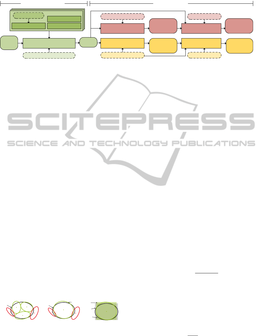
RGB

image

Segmentation

minimum run length

Averaging

regions

Heuristic

thresholds

Classification Evaluation

ground truth data

classified

regions

absolute

robustness λ

Tracking

parameters

Evaluation

tracked

regions

window length n

relative

robustness κ

result evaluationimage segmentation

Transformation

color space

window length n

min



Figure 3: Our evaluation framework. It consists of a segmentation process and two evaluation branches for measuring relative

and absolute robustness of the applied color space in combination with our segmentation algorithm.

the segmentation results signiﬁcantly differ in con-

secutive images and the current setting cannot be as-

sumed to be robust at all. Although R

may con-

tain regions with incorrect correspondences that dis-

tort the value of κ, we neglect an additional validation

step, but minimize the probability of wrongly estab-

lished correspondences by applying a highly restric-

tive parametrization to the tracking algorithm.

The ﬁnal value of κ heavily depends on the

parametrization of the selected heuristic. For exam-

ple, by simple relaxing the heuristics’s thresholds as

much as possible, the entire image plane will be rep-

resented as a single region. Although the segmenta-

tion result is not useful for any further object detection

steps, the relative robustness will be maximal with

κ = 1. In short, κ alone is not sufﬁcient for discussing

the overall robustness of a segmentation setting. For

that reason, we apply the additional evaluation branch

based on ground truth data.

4.2 Absolute Robustness

Evaluating relative robustness is done without any

foreknowledge. Evaluating absolute robustness, in

turn, is based on manually generated ground truth

data. By comparing segmentation results with ground

truth data, we estimate how robust a color space can

reproduce a desired result, e.g., under changing il-

lumination conditions. In our work, ground truth

data corresponds to a set of regions R

represent-

ing a given structure within an image. Providing that

neither camera nor objects within the image area are

moved, ground truth data has not to be generated for

region

(a)

region

(b)

overlap

(c)

Figure 4: Classiﬁcation and evaluation: (a) regions that lie

within the boundaries of region

are (b) merged into one

single region region

in order to (c) determine the overlap

between region

and its related regions by means of their

bounding boxes.

each image individually but once for an entire se-

quence. Pixels belonging to the same region are la-

beled and subsequently used to calculate the region

representation in terms of moments (cf. Section 3.2).

4.2.1 Region Classiﬁcation

The evaluation process is based on a non-exhaustive

classiﬁcation step: an extracted region region

is as-

signed to a ground truth region region

∈ R

, if its

center of mass lies within the boundaries of region

(cf. Figure 4(a)). More than one region may be as-

signed to region

, while region

may also be assigned

to more than one ground truth region. Regions that are

assigned to the same ground truth region are merged

(cf. Figure 4(b)) by adding together the correspond-

ing moments. As result of the classiﬁcation process,

each ground truth region region

∈ R

belongs to one

(possibly merged) region region

at the maximum.

4.2.2 Evaluation

The main idea of the evaluation step is to analyze the

overlap of a ground truth region region

∈ R

and

its associated region

. Instead of calculating a pixel-

precise value, we consider the overlap of the region’s

bounding boxes based on their equivalent elliptical

disks (cf. Figure 4(c)) and deﬁne the distance δ

gt,m

between those two regions as

gt,m

= 1 −

2 · A

overlap

+ A

, (6)

with A

being the area of region

’s bounding box, A

being the area of region

’s bounding box and A

overlap

being the overlapping area of both bounding boxes. If

region

does not belong to any region

, the distance

has maximum possible value of 1. The absolute ro-

bustness λ

for a framework iteration i is then deﬁned

= 1 −

∑

k=1

, (7)

with |R

| denoting the total amount of ground truth

regions and δ

being the distance (6) of the k-th

VISAPP2014-InternationalConferenceonComputerVisionTheoryandApplications

652

(a) (b)

Figure 5: Color palette of 12 different colors: (a) original,

synthetic version, (b) printed and captured by camera.

ground truth region and its assigned region. As output

value λ, we consider the averaged absolute robustness

of the last n framework iterations:

λ =

∑

i=1

. (8)

5 EXPERIMENTS

We evaluated the robustness of the four different color

spaces mentioned in Section 2 in combination with

our segmentation algorithm (Section 3.1) by consid-

ering 14 image sequences each consisting of 200 im-

ages. All sequences show exactly the same scene but

were acquired under different lighting conditions and

camera settings, respectively. The scene itself con-

sists of a palette of 12 different colors (Figure 5).

5.1 Color Space Speciﬁc Heuristics

We incorporated two different heuristics for deciding,

whether two color values are similar or not. Heuristic

is used for RGB and L

∗

. It determines sim-

ilarity of two color vectors ~µ and

ν by checking the

distance of each color channel individually:

(~µ,

ν,

τ) =











1 i f

|µ

− ν

| ≤ τ

∧

|µ

− ν

| ≤ τ

∧

|µ

− ν

| ≤ τ

0 else ,

(9)

with

τ being distinct threshold values. Heuristic h

used for HSV and LCCS. Contrary to h

, it checks the

distance of only two color channels individually:

(

υ,

ω,

τ) =







1 i f

|υ

− ω

− η| ≤ τ

∧ |υ

− ω

| ≤ τ

0 else ,

(10)

with

η =



360 i f |υ

− ω

| ≥ 180

0 else

(11)

being a correction value. Again,

τ denotes a vector of

distinct threshold values. In case of HSV color space,

the V channel is neglected. In case of LCCS, the

Cartesian coordinates (Equation 1) are transformed

into polar coordinates.

5.2 Framework Settings

The applied values for the different control values are

depicted in Table 1. The color space speciﬁc val-

ues for

τ were determined by feeding an image se-

quence with manually optimized camera parameters

and constant lighting conditions to the framework.

The threshold values were manually adjusted during

execution until the maximal possible sum κ+λ of rel-

ative and absolute robustness was identiﬁed.

Table 1: Static framework settings.

minimum run length l

min

= 5

window length n = 200

RGB thresholds (h

)

RGB

= (13,14,8)

∗

thresholds (h

)

∗

= (15,4,6)

HSV thresholds (h

)

HSV

= (13,32)

LCCS thresholds (h

)

LCCS

= (16,8)

5.3 Results

In Figure 6, relative and absolute robustness of the

14 different illuminated image scenes are plotted (cf.

short description in Table 2). Figure 6(a) shows

that relative robustness strongly differs not only be-

tween different sequences, but also for segmentation

with different color spaces applied to a single se-

quence. For sequences 1-7, where camera parameters

are manually optimized for human perception, κ is

in a high value range and differs maximal around 0.2

per sequence. This indicates that our segmentation

algorithm provides mostly equal regions over time

even at varying illumination (sequences 6 and 7). At

sequences 8-14 camera parameters are manipulated,

e.g., to get red, blue, or green cast. κ indicates that

these manipulations have heavy impact on segmenta-

tion results depending on the applied color space. At

blue cast in images, e.g., RGB and L

∗

get prob-

lems while segmentation results with HSV and LCCS

keep constant over time.

But relative robustness κ indicates only robustness

of segmented regions over time. It does not consider

whether segmentation results correspond to original

Table 2: Description of sequences considered at evaluation.

1 Manual optimized

camera parameters

8 Room light off; spot-

light from behind

2 Reduced brightness

(ﬂickering appears)

9 Room light off; spot-

light from front

3 Reduced brightness 10 Red cast

4 Shadow 11 Blue cast

5 Spotlight 12 Green cast

6 Moving shadows 13 Minimum bright-

ness of camera

7 Moving spotlight 14 Maximum bright-

ness of camera

EvaluationofColorSpacesforRobustImageSegmentation

653

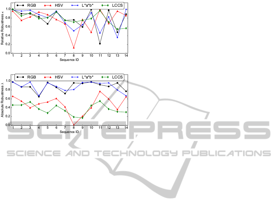
(a) Relative robustness κ.

(b) Absolute robustness λ.

Figure 6: Relative and absolute robustness results for all

sequences described in Table 2.

color segments, i.e. ground truth data. Hence, we

also have to consider absolute robustness λ depicted

in Figure 6(b). For our segmentation algorithm, it in-

dicates that robustness regarding segmentation of all

present colors under varying illumination is higher

using RGB or L

∗

than applying HSV or LCCS.

This is also conﬁrmed by the examples shown in Fig-

ure 7. For the image scene with manual optimized

camera parameters (Figures 7(a)-7(e)), we notice that

usage of RGB or L

∗

provides separate regions for

each color of the palette. In contrast, segmentation

with HSV combines, e.g., the red and orange ﬁeld as

well as the yellow and light green ﬁeld. This might

be caused by the non-linear color-ordering within the

hue-axis where yellow is only represented by a small

angle range while red and green have a higher resolu-

tion in HSV (cf. Figure 1(b)). Using LCCS provides

an even less sophisticated segmentation result where,

e.g., orange, yellow, and light green are combined.

Figures 7(f)-7(o) show that changes in illumina-

tion affect the segmentation results of all considered

color spaces. Again, RGB provides best results and

∗

also performs well. Even though L

∗

re-

gions contain less segmented pixels, regions are simi-

lar to those of RGB. Within a vision system, results

of segmentation would be used for post-processing

steps, i.e. the representation of regions would be con-

sidered. Hence, results of segmentation with RGB

and L

∗

provide similar quality in the context of a

vision system. In contrast, results of HSV and LCCS

can, e.g., no longer cover the dark colors in presence

of shadow (white areas in Figures 7(h) and 7(j)). In

case of segmentation with HSV, this might be an im-

plementation issue because within HSV we do not

consider values positioned in a certain range around

the vertical axis of the color cylinder to avoid noised

gray values. Consequently, colors that appear almost

gray or even black were neglected by segmentation

using HSV. This has also negative effects regarding

the absolute robustness because the distance function

introduced in Equation 6 returns δ = 0 for these miss-

ing color ﬁelds.

In presence of an additional spotlight (Fig-

ures 7(k)-7(o)), the yellow ﬁeld of the palette is too

much affected by reﬂections and therefore appears

almost white in the original image. Nevertheless,

segmentation with all considered color spaces except

LCCS extracts a region that at least partially covers

this area. Within segmentation using LCCS, all orig-

inally green and yellow color ﬁelds of the palette are

fused to one region with kind of mint green as average

color. Again, RGB and L

∗

provide best results.

6 CONCLUSIONS AND

OUTLOOK

In this paper, we presented our color-based segmen-

tation approach and evaluated its robustness in com-

bination with different color spaces. To investigate

the robustness of a speciﬁc segmentation setting, we

introduced our framework that directly works on our

statistical region representation. In this context, the

out-standing feature of the framework is the evalu-

ation of two different types of robustness: relative

robustness and absolute robustness. Relative robust-

ness is evaluated by tracking regions across consecu-

tive images, while absolute robustness is evaluated for

each frame individually based on manually generated

ground truth data.

With the evaluation of our segmentation algo-

rithm, on the one hand we proved the relative and

absolute robustness as a signiﬁcant quantitative mea-

sure for robustness. On the other hand, we showed

that in our artiﬁcial setting the presented segmenta-

tion algorithm performs best using RGB color space.

Nevertheless, for some situations the segmentation

approach provided better results using other color

spaces like L

∗

or HSV.

In our future work, we want to use the evaluation

framework for automatically calibrating our segmen-

tation algorithm as well as adapting the threshold val-

ues used by our heuristics during execution time. Fur-

thermore, we want to switch from artiﬁcial scenes to

more realistic scenarios while appropriately adjusting

VISAPP2014-InternationalConferenceonComputerVisionTheoryandApplications

654

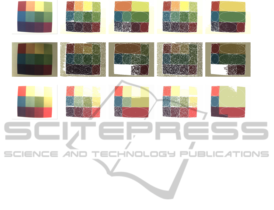
(a) Room light. (b) RGB. (c) HSV. (d) L

∗

. (e) LCCS.

(f) Shadow. (g) RGB. (h) HSV. (i) L

∗

. (j) LCCS.

(k) Spotlight. (l) RGB. (m) HSV. (n) L

∗

. (o) LCCS.

Figure 7: Original images and corresponding segmentation results using different color spaces. Images captured under room

light (a-e; sequence 1), with additional shadow (f-j; sequence 4), and with a spotlight (k-o; sequence 10).

the functionality of our evaluation framework, if nec-

essary. Aside from evaluating robustness of segmen-

tation results, we additionally intend to investigate if

the presented approach can be used for comparing im-

ages not on pixel level but on region level.

ACKNOWLEDGEMENTS

This work was partially supported by the German Research

Foundation (DFG) within the Collaborative Research Cen-

ter “On-The-Fly Computing” (SFB 901).

REFERENCES

Blas, M., Agrawal, M., Sundaresan, A., and Konolige, K.

(2008). Fast color/texture segmentation for outdoor

robots. In IEEE/RSJ International Conference on

Intelligent Robots and Systems (IROS), pages 4078–

4085.

Busin, L., Shi, J., Vandenbroucke, N., and Macaire, L.

(2009). Color space selection for color image segmen-

tation by spectral clustering. In IEEE International

Conference on Signal and Image Processing Applica-

tions (ICSIPA), pages 262–267.

Finlayson, G. D., Drew, M. S., and Lu, C. (2009). Entropy

minimization for shadow removal. Int. J. Comput. Vi-

sion, 85(1):35–57.

Freixenet, J., Mu

noz, X., Raba, D., Mart

ı, J., and Cuf

ı,

X. (2002). Yet another survey on image segmenta-

tion: Region and boundary information integration. In

Proceedings of the 7th European Conference on Com-

puter Vision (ECCV), pages 408–422.

Hu, M.-K. (1962). Visual pattern recognition by moment

invariants. IEEE Transactions on Information Theory,

8(2):179–187.

Jungmann, A., Kleinjohann, B., Kleinjohann, L., and

Bieshaar, M. (2012). Efﬁcient color-based image seg-

mentation and feature classiﬁcation for image pro-

cessing in embedded systems. In Proceedings of the

4th International Conference on Resource Intensive

Applications and Services (INTENSIVE), pages 22–

29.

Jungmann, A., Stern, C., Kleinjohann, L., and Kleinjohann,

B. (2010). Increasing motion information by using

universal tracking of 2d-features. In Proceedings of

the 8th IEEE International Conference on Industrial

Informatics (INDIN), pages 511–516.

Khanal, B., Ali, S., and Sidib, D. (2012). Robust road

signs segmentation in color images. In Proceedings of

the 7th International Conference on Computer Vision

Theory and Applications (VISAPP), pages 307–310.

Mogelmose, A., Trivedi, M., and Moeslund, T. (2012).

Vision-based trafﬁc sign detection and analysis for in-

telligent driver assistance systems: Perspectives and

survey. IEEE Transactions on Intelligent Transporta-

tion Systems, 13(4):1484–1497.

Russell, S. and Norvig, P. (2010). Artiﬁcial Intelligence - A

Modern Approach. Pearson, 3 edition.

Szeliski, R. (2011). Computer Vision - Algorithms a. Appli-

cations. Springer.

Unnikrishnan, R., Pantofaru, C., and Hebert, M. (2007). To-

ward objective evaluation of image segmentation al-

gorithms. IEEE Transactions on Pattern Analysis and

Machine Intelligence, 29(6):929–944.

Vandenbroucke, N., Macaire, L., and Postaire, J.-G. (2003).

Color image segmentation by pixel classiﬁcation in

an adapted hybrid color space: application to soccer

image analysis. Computer Vision and Image Under-

standing, 90(2):190–216.

Yang, U., Kim, B., and Sohn, K. (2009). Illumination in-

variant skin color segmentation. In 4th IEEE Con-

ference on Industrial Electronics and Applications

(ICIEA), pages 636–641.

EvaluationofColorSpacesforRobustImageSegmentation

655