Calibration and 3D Ground Truth Data Generation with Orthogonal

Camera-setup and Refraction Compensation for Aquaria in Real-time

Klaus M

uller, Jens Schlemper, Lars Kuhnert and Klaus-Dieter Kuhnert

Institute of Realtime Learning Systems, Department of Electrical Engineering and Computer Science, University of Siegen,

olderlinstr. 3, 57076 Siegen, Germany

Keywords:

Calibration, Fish Tank, Refraction, 3D-model, Tracking, Vision, Segmentation.

Abstract:

In this paper we present a novel approach to generate precise 3D ground-truth data considering the refraction

of the ﬁsh tank. We used an accurate and easy-to-handle calibration method to calibrate two orthogonally

aligned high-resolution cameras in real-time. For precise ﬁsh shape segmentation we combined two different

background subtraction algorithms, which can also be trained while ﬁsh are swimming inside the aquarium.

The presented approach takes also shadow segmentation removal and mirroring into account. For refraction

compensation at the air-water border we developed an algorithm which calculates the ray-deﬂection of every

shape-pixel and compute the 3D-model in real-time.

1 INTRODUCTION

In ﬁsh behaviour studies computer vision is a well

known tool to observe ﬁsh’s position and movements.

One of the main research areas in this scope is the

study of mate-choice. The classical approach for mate

choice studies is laborious and time-consuming, due

to the fact, that real mate’s behaviour is undeﬁned and

hardly repeatable.

The presented work is part of an interdisciplinary

project between computer science and biology. The

aim of the project is to create a virtual ﬁsh which in-

teracts with real ﬁsh for conducting strictly-controlled

behavioural mate-choice-studies. At ﬁrst ﬁsh’s move-

ments and behaviour have to be analysed with the help

of a computer vision system. In the sequel the gath-

ered information is used to create a photo-realistic

simulation of ﬁsh and their behaviour. The used ﬁsh

species is sailﬁn molly (see Figure 1), which has a size

of 4 to 10 cm and is able to move quite quickly and

rather abruptly. Especially, its quick movements place

special demands on the computer vision system.

In a future step, a ﬁsh model will be created with

Figure 1: Sailﬁn mollies.

the help of the gathered shape, movement and be-

haviour information of the species. This steerable

virtual ﬁsh may be used by the behaviour scientists

to conduct ﬁsh-behaviour experiments under strictly

controlled conditions. With the help of the track-

ing information of the real ﬁsh the virtual ﬁsh pro-

jected onto a screen can react to and also interact

with the real ﬁsh. Furthermore the model will be

utilised to build a tracking system based on a model-

based approach using an appearance model of the ﬁsh

(analysis-by-synthesis). The analysis-by-synthesis

method allows to track the ﬁsh’s 3D-position and 3D-

deformation by using only one camera. Due to the

model’s information about the ﬁsh’s movements the

algorithm renders the most probable image of the vir-

tual ﬁsh and compares this to the captured image of

the real ﬁsh. This step is repeated until the rendered

image becomes undistinguishable from the captured

image. As a result the algorithm provides the best ﬁt

model parameters and consequently a complete ﬁsh

description in 3D.

In this paper we describe the ﬁrst period of this

project. Besides the setup of the computer vision sys-

tem, we also developed a segmentation and recon-

struction system to get precise ground truth data of

the ﬁsh’s position, pose and movement under consid-

eration of refraction at the air-water-boarder. On the

one hand this is the precondition for creating a virtual

ﬁsh, on the other hand this allows to quantitatively

evaluate the results stemming from the new analysis-

626

Müller K., Schlemper J., Kuhnert L. and Kuhnert K..

Calibration and 3D Ground Truth Data Generation with Orthogonal Camera-setup and Refraction Compensation for Aquaria in Real-time.

DOI: 10.5220/0004743506260634

In Proceedings of the 9th International Conference on Computer Vision Theory and Applications (VISAPP-2014), pages 626-634

ISBN: 978-989-758-009-3

 2014 SCITEPRESS (Science and Technology Publications, Lda.)

by-synthesis approach later on.

The future system will be able to handle multiple

ﬁsh. Due to the fact that the main focus of this pa-

per lies on calibration, segmentation and refraction-

compensation, we conduct our tests with a single ﬁsh

and do not take occlusion (ﬁsh-ﬁsh) into account.

2 BACKGROUND AND

METHODS

For the following experiments we use a ﬁsh tank with

the size of 600 mm x 300 mm x 300 mm.

2.1 Computer Vision Setup

Due to the fact that computer vision systems be-

came more powerful and easier to use their num-

ber in animal behaviour studies has increased during

the last years (Delcourt et al., 2012). Especially in

ﬁsh-behaviour projects it is a very important tool to

observe ﬁsh’s movement, position and consequently

its behaviour. During the last years besides two-

dimensional tracking systems (e.g. (Fontaine et al.,

2008)) also three-dimensional tracking systems have

been established ((Zhu and Weng, 2007); (Butail and

Paley, 2012)). For the latter one different types of vi-

sion systems are used in ﬁsh behaviour studies.

2.1.1 Camera Setup and Illumination

The method described in Laurel et al. (Laurel et al.,

2005) is based on ﬁsh shadows. They installed two

lamps above the aquarium and recorded the ﬁsh and

their shadows with one camera. With the help of

trigonometric computations they calculated the ﬁsh’s

positions. For increasing numbers of ﬁsh this kind

of tracking system is not suitable caused by the oc-

clusions of multiple shadows. Zhu and Weng (Zhu

and Weng, 2007) extended their ﬁsh tank with mir-

rors above and on the left side of the aquarium. Be-

sides the front view the camera placed in front of

the aquarium also recorded the mirrored top and left

view. By doing so this system is also suitable for big-

ger ﬁsh groups. Butail and Paley (Butail and Paley,

2012) used three orthogonal cameras, placed above,

in front and on the left side of the ﬁsh tank. They

reconstructed ﬁsh bodies by extracting ellipses from

ﬁsh images of two cameras and combining them to an

ellipsoid in a post processing step. The left camera

was used for validation of the tracking result.

For our future analysis-by-synthesis tracking-

approach we need high resolution coloured pictures

of the ﬁsh. Additionally initial tests showed that the

Figure 2: Camera system with illumination. The ﬁsh tank

is equipped with red marker balls.

ﬁsh can turn their body within 100 ms around 180

◦

what places special demands on the camera. For that

reasons we chose two gigabit ethernet color cameras

(Allied Vision Technologies, Prosilia GT1910c)

with a resolution of 1920 x 1080 and with a frame

rate of 57 frames per second. The cameras were

synchronised by a hardware trigger and connected

over gigabit ethernet to a stationary PC (quad core

CPU Intel i5-2320 3 Ghz, two Gigabit Ethernet cards,

RAID0 system). The cameras produce 220 MB of

raw data per second. For 3D calculation we chose

a camera setup similar to (Butail and Paley, 2012).

We mounted the cameras on a ﬁxed frame. The ﬁrst

one was placed above and the second one in front of

the ﬁsh tank. For illumination we chose LED stripes

placed on both sides at an angle of 45

◦

above the

tank (see Figure 2). In contrast to other systems in

this scope (Fontaine et al., 2008; Butail and Paley,

2012; Yamashita et al., 2011) our system is real-time

capable.

2.1.2 System Infrastructure

Given that the ﬁnal system will be used for interactive

ﬁsh behaviour studies in future it will consist of sev-

eral subsystems placed on different computers. Based

on this assumption every part of the system (track-

ing system, observer control system and 3D-ﬁsh en-

gine) has to communicate with each other in real time.

Owing to this fact a suitable communication system

is necessary. Due to our former positive experience

with the robot operating system ROS (Quigley et al.,

2009) in context of distributed systems and multi sen-

sor networks (Kuhnert et al., 2012) we decided to use

this system in this project, too. Besides, the easy

communication over Ethernet between all sensors and

software modules, ROS includes a huge toolbox for

Calibrationand3DGroundTruthDataGenerationwithOrthogonalCamera-setupandRefractionCompensationfor

AquariainReal-time

627

recording and manipulating sensor data.

2.2 Camera Calibration

For three-dimensional object-tracking with two cam-

eras accurate camera calibration is very essential.

Especially in ﬁeld of ﬁsh-tracking in aquariums re-

fraction places special demands on the calibration

method. Butail and Paley (Butail and Paley, 2012)

used in their paper the camera calibration toolbox of

Matlab (Bouguet, 2004). For calibration they ﬁlmed

a planar checkerboard underwater at different orienta-

tions. Their method does not take the air-water refrac-

tion into account and they assumed that this caused in-

accuracies. Yamashita et al. (Yamashita et al., 2011)

used omni-directional stereo cameras for underwa-

ter sensing. These were placed above each other in

an acrylic cylindrical waterproof case. For refrac-

tion compensation Yamashita et al. used an optical

ray tracing technique. For our purpose it is very im-

portant that the calibration system is easy and fast to

handle hence the experiment conductors can calibrate

it themselves after an accidental camera displace-

ment during the experiments. For the intrinsic camera

calibration and radial lens distortion we applied the

widely-used OpenCV calibration tools (opencv.org,

2013). Given that the internal camera parameter does

not get changed during the experiments, these were

calculated once in our institute. For extrinsic calibra-

tion we chose external, easy to mount markers on the

ﬁsh tank. These can be used to calculate the cam-

era position according to the ﬁsh tank’s coordinate

system. For markers we used red golf balls. With

a CNC-milling machine we cut edges in the balls to

ﬁt it accurately to the ﬁsh tank corners. We ﬁxed six

balls on two sides of the ﬁsh tank, so that four balls

are visible in every camera view (see Figure 2).

2.2.1 Extrinsic Camera Calibration

Extrinsic camera calibration is a well studied prob-

lem in computer vision and several tools are available

on the market. The most calibration methods esti-

mate the homography between a model plane, which

has distinctive known feature points (like a checker-

board), and its image [e.g. (ZHANG, 2000)]. These

methods are based on a pinhole camera model and

do not take any kind of refraction into account. For

that reason these methods cause inaccuracies in ap-

plications with cameras outside of a water ﬁlled ﬁsh

tanks. For reducing these inaccuracies it is possible

to put the model plane inside the water ﬁlled aquar-

ium and calibrate the cameras [e.g. (Butail and Paley,

2012)]. In this case the algorithm balances the refrac-

tion by shifting the estimated camera position behind

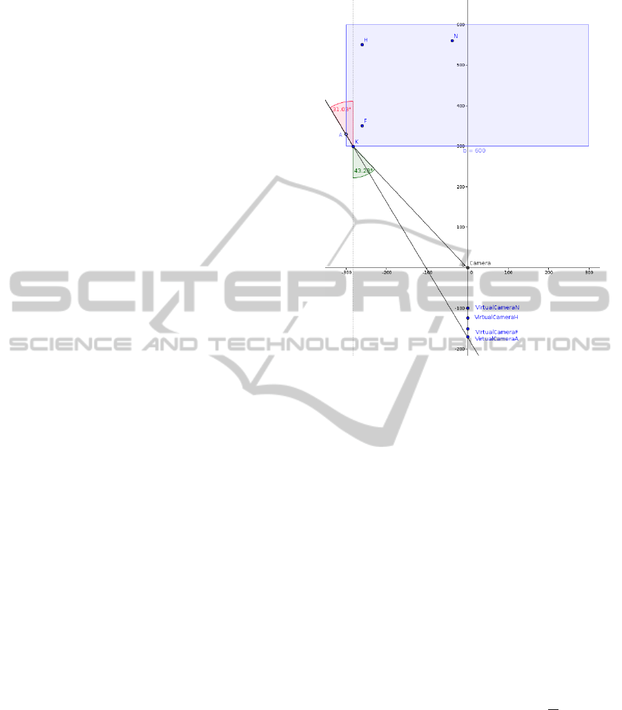
Figure 3: Extrinsic Camera calibration without consider-

ing refraction. The estimated camera position VirtualCam-

era[H,F,A,N] depends on the referred object point inside the

water-ﬁlled aquarium (A, F, H and N) and is not unique.

the real camera position what compensates the refrac-

tion locally. This also reduces the error globally but

does not deliver a distinct camera position. As shown

in Figure 3 the estimated camera position depends on

the location of the referred point.

For that reason we split the calibration in two

parts. In the ﬁrst part we calibrate our cameras re-

ferring to the ﬁxed balls outside of the aquarium. In

the second part we calculate the refraction of every

single camera ray using the refraction law.

Predeﬁnition

For the following calculations we assume that:

• The vector ~x has the components (x

)

• A normalized vector is deﬁned as ˆx =

|~x|

• ~x

1,2

is a short form of ~x

and ~x

• In the following the indices 1 and 2 refer to Cam-

era 1 and Camera 2.

Camera Calibration with Marker Balls

Based on shapes of the balls and their centre positions

ﬁxed to the tank corners we assume that the centre

VISAPP2014-InternationalConferenceonComputerVisionTheoryandApplications

628

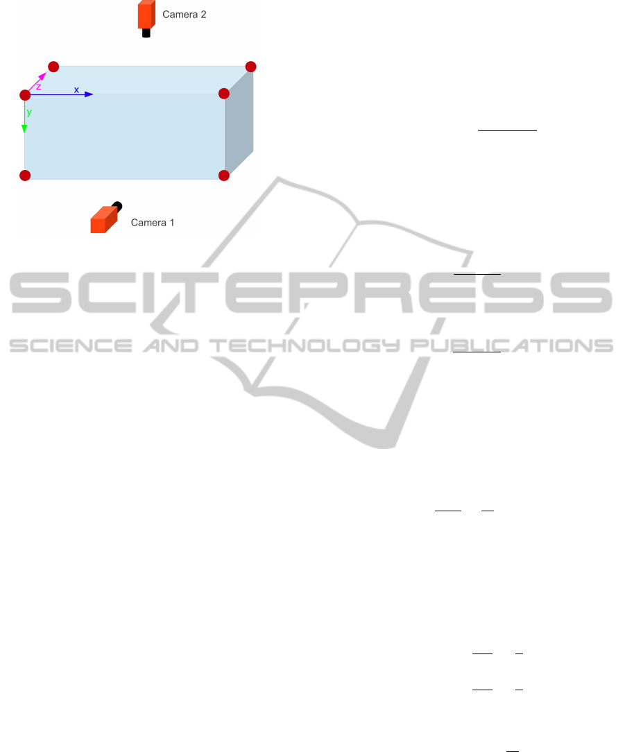
Figure 4: Coordinate system of the ﬁsh tank.

of the balls image plain projection also describes the

camera ray through the tank corners. We also know

the physical dimensions of the ﬁsh tank and assume

that the xy-plane of our coordinate system lies on

the front window with z-axis heading to the back of

the tank (see Figure 4). As the balls are painted red

we use a colour-based blob detection algorithm for

marker identiﬁcation. By calculating the moment of

the segmented balls we get the centre of them. In our

tests the standard deviation of the ball centres with

100 samples was below 0.05 pixels.

With the help of four 3D-2D point correspon-

dences obtained from the former step, we calculate

positions and poses of the cameras. We solve this

problem by using the analytic method presented in

(Gao et al., 2003). Gao et al. used an algebraic ap-

proach to solve the perspective-three-point problem.

The algorithm delivers the camera calibration matri-

ces C

and C

according to the coordinate system

shown in Figure 4. The camera calibration matrices

are deﬁned as

1,2

= (R

1,2

) (1)

with rotation matrix R

1,2

and translation vector t

1,2

Ray Refraction Calculation

In the following calculation we disregard the refrac-

tion of the aquarium-glass given that the caused shift-

ing error is less than 0.12 mm in the worst case and is

negligible.

For calculating the refraction we trace the ray

starting at the projection center of the camera, passing

the air-water border through

1,2

and ﬁnally ending up

at the object. The starting point (projection center)

1,2

of the ray is deﬁned as follows:

1,2

= −R

1,2

−1

1,2

(2)

We get the ray ~x

1,2

, which starts at the camera project

center, by multiplying the inverse of the projection

matrix with the according 2D point x

. Given that the

projection matrix is singular, we invert it using singu-

lar value decomposition.

ˆx

1,2

= C

−1

1,2

−

1,2

−

1,2

(3)

For getting the ray piercing point at the air-water bor-

der we compute the length of the ray between

and

. Due to the fact that the hit plane for the ﬁrst camera

is identical to the x-y plane and for the second camera

parallel to the x-z plane, we simplify the calculation.

1,2

describes the length factor:

− x

. (4)

For the second camera we have to consider the water

level w, which is measured manually:

− w

− x

. (5)

Finnally we use c

1,2

to compute the intersection point

1,2

= c

1,2

( ~x

1,2

−

1,2

) +

1,2

. (6)

The refraction of rays passing from one medium to

another is deﬁned by

sinα

sinβ

(7)

with the indices of refraction n

and n

For getting α we calculate the angle between the cam-

era ray~x

and the front side of the tank and the camera

ray~x

and the water plane. Since these planes are par-

allel to the coordinate system planes we simplify the

calculation.

= sin

−1

(

|~x

) −

(8)

= sin

−1

(

|~x

) −

(9)

Based on (7) we get

= sin

−1

(sinα

1,2

). (10)

The ray is turned in

1,2

around the axis ~a

1,2

. ~a

1,2

perpendicular to the plane between~x

1,2

and the center

ray of the cameras ~c

1,2

. c

describes the center pixel

of the cameras.

1,2

= (C

1,2

−1

) ×~x

1,2

(11)

Calibrationand3DGroundTruthDataGenerationwithOrthogonalCamera-setupandRefractionCompensationfor

AquariainReal-time

629

Figure 5: Ray refraction. γ is the angle of refraction.

We calculate a rotation matrix R

1,2

with the help of

the normalized vector ˆa

1,2

. As shown in Figure 5 the

ﬁnal turning angle γ is deﬁned

γ = β− α. (12)

1,2









with

= ˆa

(1 − cosγ) + cos γ

= ˆa

ˆa

(1 − cosγ) + ˆa

sinγ

= ˆa

ˆa

(1 − cosγ) − ˆa

sinγ

= ˆa

ˆa

(1 − cosγ) − ˆa

sinγ

= ˆa

(1 − cosγ) + cos γ

= ˆa

ˆa

(1 − cosγ) + ˆa

sinγ

= ˆa

ˆa

(1 − cosγ) + ˆa

sinγ

= ˆa

ˆa

(1 − cosγ) − ˆa

sinγ

= ˆa

(1 − cosγ) + cos γ

(13)

Finally we get the refracted ray ~x

1,2

. It starts at

1,2

= R

1,2

ˆx

1,2

(14)

2.3 Segmentation

Fish segmentation is an important part of our work,

because the 3D model generation is based on the ﬁsh

shape information. Therefore, we use a very precise

segmentation method which is also robust against ﬁsh

shadows. Additionally it is simple and fast to ini-

tialise. In the future behaviour studies the ﬁsh need

a period of acclimation in the ﬁsh tank. With our ap-

proach we can generate the background during the ac-

climation time automatically.

As the environment of the ﬁsh and also the

cameras are static the most projects in this scope

used background subtraction methods for ﬁsh-

segmentation (Delcourt et al., 2012). Fontaine et al.

(Fontaine et al., 2008) used a semi-automated routine

for an initial detection of ﬁsh. They took the ﬁrst

video frame and marked the region around the ﬁsh.

With the help of a Matlab function they erased the

ﬁsh and estimated the background model for segmen-

tation.

In our approach we also use background subtrac-

tion methods for ﬁsh segmentation. We combine two

different background subtraction methods and bene-

ﬁt from the advantages of each. On the one hand we

use the Gaussian Mixture-based subtraction method

(GMS) (Zivkovic, 2004). The GMS method is an

adaptive method which adapts the background over

time. Especially in scenes with moving foreground

objects it is well suited. But if the objects stay at

the same place the method starts to add the object

to the background. In our project that caused errors

especially if ﬁsh stay for a longer time at the same

place. The detected foreground objects starts to shrink

as seen in Figure 6. On the other hand we use a

codebook based subtraction method (CB) (Kim et al.,

2005). The background of this method is static after

initialization and also staying objects get segmented.

Normally the background generation of CB is done

with background images without foreground objects.

Since we initialize the background during ﬁsh

swimming inside the tank we split the process into

two steps. In the ﬁrst step we initialize the CB back-

ground by using the GMS method. In the second step,

the CB method creates a precise foreground.

In the ﬁrst step the GMS method normally ﬁnds at

least a small part of the ﬁsh like a ﬁn as it is constantly

moving and cannot be confused with background.

With this information we create a mask around the

GMS found foreground objects. Based on center c

of the contour n, we build a rectangle R

around c

with ﬁxed width w and height h values, so that the

supposed ﬁsh body is covered completely. This mask

is applied during computation of the CB background.

Background areas which are covered by the mask do

not get updated.To ensure that every background pixel

is updated sufﬁciently we count the updates on ev-

ery pixel. Once every pixel is updated n times, the

background generation is ﬁnished and the segmenta-

tion starts.

Finally we apply a contour-searching algorithm to

the CB foreground image and store the contour areas

of camera 1 A

and camera 2 A

2.3.1 Contour Referencing and Mirroring

Avoidance

For the 3D ground truth model generation we need

pairs of contours (A

) from both cameras, which

describe the same object. Owing to the fact, that we

VISAPP2014-InternationalConferenceonComputerVisionTheoryandApplications

630

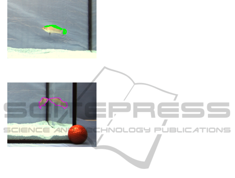
Figure 6: Shrunken foreground contour. The ﬁsh stayed at

the same place for a longer time - as a result the foreground

created by GMS shrinks.

Figure 7: Mirrored ﬁsh. The ﬁsh on the left is mirrored in

the right window.

know the path of every camera ray (see section 2.2)

we calculate the distance between the camera rays~x

and ~x

) of two potential referring contours A

and

In order to measure the distance between referring

pixel rays (facing the same three dimensional point),

we choose the pixel x

and x

with the lowest x-value

of the contour. With equation (14) we get the ray of

and x

and calculate the distance between the two

lines. The calculation sequence is described in the

following:

for (i = 0; i < foundContours_cam1; i++)

{

pixMinX_Cam1 =

search pixel with min x of

foundContours_cam1(i);

rayCam1 = calculate ray of pixMinX_Cam1;

for(j = 0; j <foundContours_cam2; j++)

{

pixMinX_Cam2 =

search pixel with min x of

foundContours_cam2(j);

rayCam2 = calculate ray of pixMinX_Cam2;

if(distance(rayCam1, rayCam2) < epsilon)

store pair(foundContours_cam1(i),

foundContours_cam2(j));

}

The stored pair of contours describes the same three-

dimensional object.

As shown in Figure 7 the ﬁsh is mirrored when it

comes up to the aquarium glass. In consequence the

segmentation system also segments the mirrored ﬁsh.

With the help of the described technique these mir-

rored contours get ignored. By matching the contours

of both cameras, no suitable contour is found for the

mirrored one and it gets deleted.

2.3.2 Shadows

As seen in Figure 8 another problem which occurs

during segmentation is shadow segmentation. We

solve that problem by adjusting the CB subtraction

method. For every pixel the CB background stores

one or more ranges of values for every color channel.

Only if a tested pixel ﬁts in all of this ranges, it will

be accepted as background. Because of this we can

expend the luminance channel range of CB, without

assessing a pixel as background by mistake. As an

effect luminance based changes have only slight in-

ﬂuence on the ﬁnal foreground image.

2.4 3D Ground Truth Model

Generation

For our future work, we need a precise 3D model in

which we can ﬁt our own created ﬁsh model. Partic-

ular attention has to be turned to the bending along

the roll-axis of the ﬁsh, so that we are able to re-

construct the movement of the ﬁsh precisely. This is

given by the orthogonal camera setup with a camera

above the tank. On the other side with this setup, it

is not possible to ﬁnd texture based reference points

like in stereo-vision setups. Consequently our method

creates a box type ﬁsh model that sharply reconstructs

the bending along the roll axis and the position.

At ﬁrst we create a set of triangles along the ﬁsh’s

contour rays ~x

from camera 1. n describes the ray

number. ~x

and ~x

n+1

are neighbouring rays.

is the starting point of ray ~x

. Given that we want

to create a model inside the ﬁsh tank we deﬁned an

ending point of ray ~x

= ˆx

l +

(15)

l is the maximal ray length inside the tank. The tri-

angles along the contour are deﬁned as follows. For

Calibrationand3DGroundTruthDataGenerationwithOrthogonalCamera-setupandRefractionCompensationfor

AquariainReal-time

631

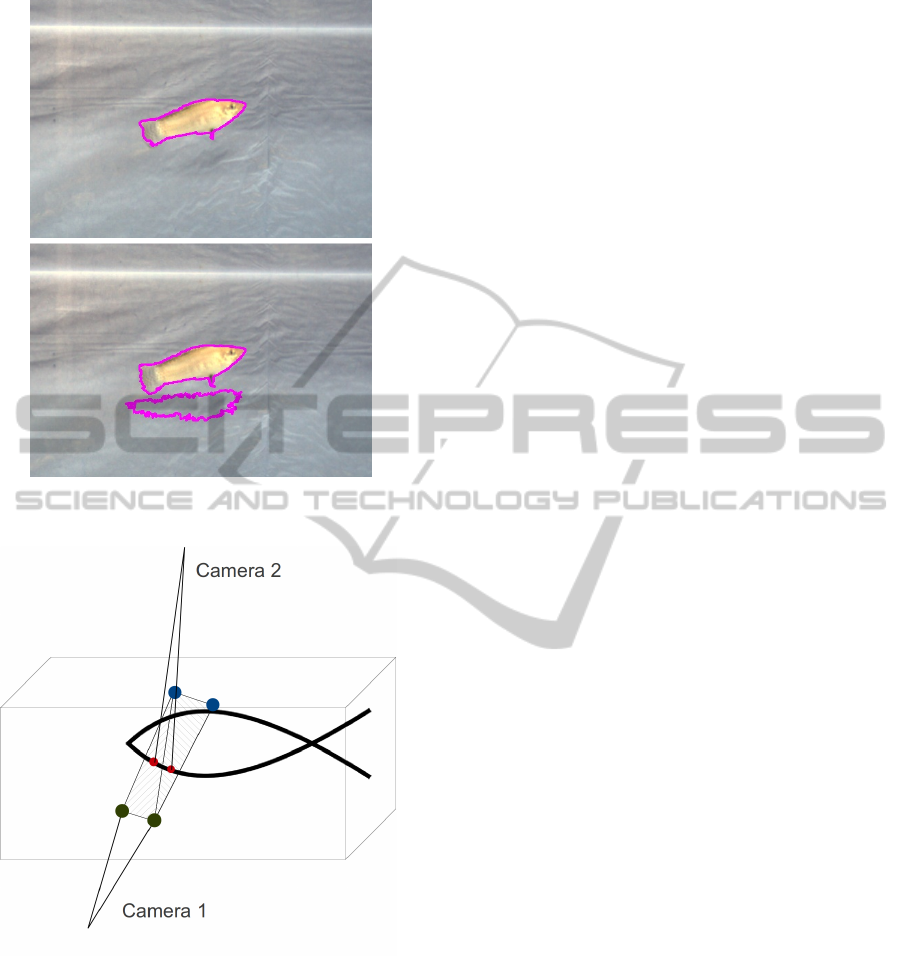
Figure 8: Fish shadow. Segmentation with (upper image)

and without (lower image) shadow avoidance.

Figure 9: 3D calculation. The contour rays of camera 1 in-

tersect with the front window (green points) pass through

the tank and end up at the back window of the tank (blue

points). The red points represent the intersection point of

contour rays of camera 2 and the spanned triangles of cam-

era 1.

each ray we construct two triangles:

= 4(

,~e

n+1

)

= 4(~e

n+1

,~e

n+1

)

(16)

The triangles border the ﬁsh contour along the op-

tical axis of camera 1 so that we have a tube in shape

of a ﬁsh starting at the front side and ending up at the

back side of the tank.

For getting the ﬁnal 3D ground truth model of

the ﬁsh we use the ﬁsh contour information from the

second camera. We calculate the intersection points

of the refracted rays ~x

(camera 2) and the trian-

gle mesh created in the former step (see Figure 9).

The calculation sequence is described in the follow-

ing pseudo code:

for (i = 0; i < n_ray2; i++)

{

for(j = 0; j < n_ray1; j++)

{

if ray2_i intersect triangle1_j

calculate intersectionPoint;

store intersectionPoint;

if ray2_i intersect triangle2_j

calculate intersectionPoint;

store intersectionPoint;

}

For testing of intersection and calculating the in-

tersection point we use the ray-triangle method of

oller and Trumbore which is explained in (Moeller

and Trumbore, 1997).

Finally the detected set of 3D points represents an

abstract model of the ﬁsh. This model combines be-

sides the absolute position all important moving and

bending parameters of the ﬁsh.

3 RESULTS

In the following we present the results of calibration,

segmentation and 3D ground truth data generation.

3.1 Calibration

In order to test the calibration a reference objects

(cuboid of aluminium) was manufactured with a pre-

cision of 0.01 mm. We placed it in different locations

and orientations in the ﬁsh tank and recorded images

of it. Afterwards we manually selected the corners of

the cuboid in both camera images. Based on the pixel

values of the corners we calculated the world coordi-

nates using the extrinsic camera calibration. Finally,

we measured the distance between the corners using

the method described in Section 2.4. In our tests we

got a mean distance (relative) error of 0,31 mm with

a standard deviation of 0,22 mm.

For measuring the absolute position error we

placed the cuboid in the deﬁned corners of the aquar-

ium and measured the position of the cuboid inner

corners as described above. We got a maximal (abso-

lute) error of 2.1 mm. By deactivating the refraction

compensation the error increased to 12.6 mm.

VISAPP2014-InternationalConferenceonComputerVisionTheoryandApplications

632

3.2 Segmentation

We tested the previously shown segmentation method

under various illumination conditions, with ﬁsh

of different size and with different ground sub-

strates(sand,grit). The initialization of the CB back-

ground subtraction with the help of the GMS yielded

in reasonable results. Depending on the number of

ﬁsh the time of initialization varied. In our tests

we stopped the initial process after every background

pixel was updated at least 50 times. In the worst case

the initialisation took up to 60 s. The implemented

shadow removal also worked well. During our tests

we adjusted the illumination threshold of our back-

ground subtraction regarding to the used illumination.

We ﬁgured out that a high threshold value (very dark

shadows) also inﬂuences the segmentation negatively.

Especially transparent tail ﬁns of female ﬁsh were not

segmented completely under the described circum-

stances.

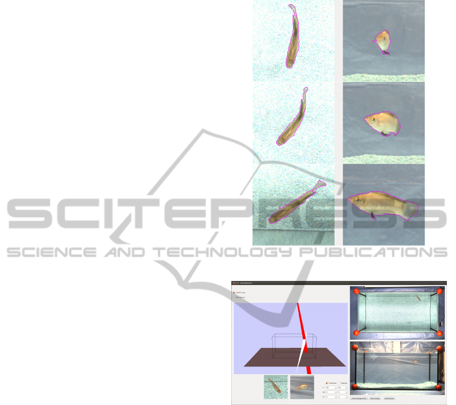
Figure 10 shows some results of the segmentation.

As seen in the images the ﬁsh was segmented in the

images of both cameras. Since the background of the

front camera image was more homogeneous than the

background of the upper camera, the segmented con-

tour is smoother. The lateral ﬁns of the ﬁsh are trans-

parent and were not detected by the algorithm.

3.3 3D Ground Truth Model

For visualisation and validation of the 3D ground

truth data we developed a 3D viewer, which visual-

izes the camera rays in real time (see Figure 11). The

two camera projection centers are placed in front and

above the ﬁsh tank. From there the rays are refracted

at the air-water border and run through the aquarium.

The skew rays of the two cameras approximately in-

tersect inside the aquarium. To get the approximated

intersection point, we computed the shortest line be-

tween the two skew rays and calculated the center

point of the line. This represents the observed 3D

object point. As unit of error measurement we de-

ﬁned the distance between the most left rays of ﬁrst

and second cameras’ pixel contours. In case of a ﬁsh

we measured the distance between the pixel rays of

the snout. In our test a ﬁsh was swimming from one

side of the tank to the other side. The measured mean

distance between the two rays was 0.64 mm with a

standard deviation of 0.72 mm.

4 CONCLUSIONS

In this paper we presented a novel approach for gen-

Figure 10: Segmented ﬁsh in different pose from the upper

camera (left) and the front camera (right).

Figure 11: Visualisation tool. On the left it shows the vir-

tual 3D ﬁsh tank with the contour rays of the upper camera

(red) and the front camera (white). The referring images are

shown on the right side.

erating 3D ground truth data of ﬁsh in an aquarium

considering refraction in real time. With regards to

the utilization in ﬁsh behavioural studies a well op-

erating and easy to handle application was requested.

Taking the water-refraction into account, we achieve

a very precise extrinsic camera calibration. As indi-

cated in the results, the relative exactness of the pre-

sented method is about +/- 0.3 mm. The absolute po-

sition error of 2.1 mm is based on the precision of

the aquarium manufacturing. It can be decreased by

increasing the precision of the aquarium manufactur-

ing.

Furthermore, we established a segmentation

method by combining two background subtraction

methods – one based on codebook and one adapted

Calibrationand3DGroundTruthDataGenerationwithOrthogonalCamera-setupandRefractionCompensationfor

AquariainReal-time

633

from the Gaussian Mixture-based background sub-

traction method. By doing so, we are able to initialize

the background with ﬁsh in the tank. In addition, it

is possible to exclude mirror images and shadows of

the ﬁsh easily. The advantages of this approach lie in

the high precision combined with an easy utilization

in real time. In the future, based on these ground truth

data we can adopt ﬁsh’s behaviour and movements for

virtual ﬁsh; furthermore the data can serve as a con-

trol for the ﬁnal analysis-by-synthesis system.

ACKNOWLEDGEMENTS

The presented work was developed within the scope

of the interdisciplinary, DFG-funded project “virtual

ﬁsh” of the Institute of Real Time Learning Systems

(EZLS) and the Department of Biology and Didactics

at the University of Siegen.

REFERENCES

Bouguet, J.-Y. (2004). Camera calibration toolbox for mat-

lab. http://www.vision.caltech.edu/bouguetj/calibdoc/

[26.08.2013].

Butail, S. and Paley, D. A. (2012). Three-dimensional

reconstruction of fast-start swimming kinematics of

densely schooling ﬁsh. Journal of The Royal Society

Interface, 9:77–88.

Delcourt, J., Denoel, M., Ylieff, M., and Poncin, P. (2012).

Video multitracking of ﬁsh behaviour: a synthesis and

future perspectives. Fish and Fisheries, 14:186–204.

Fontaine, E., Lentink, D., Kranenbarg, S., Mueller, U. K.,

van Leeuwen, J. L., Barr, A. H., and Burdick, J. W.

(2008). Automated visual tracking for studying the

ontogeny of zebraﬁsh swimming. Journal of Experi-

mental Biology, 211:1305–1316.

Gao, X. S., Hou, X. R., Tang, J., and Cheng, H. F. (2003).

Complete solution classiﬁcation for the perspective-

three-point problem. IEEE Transactions on Pattern

Analysis and Machine Intelligence, 25(8):930–943.

Kim, K., Chalidabhongse, T. H., Harwood, D., and Davis,

L. (2005). Real-time foreground–background seg-

mentation using codebook model. Real-time imaging,

11(3):172–185.

Kuhnert, L., Thamke, S., Ax, M., Nguyen, D., and Kuhnert,

K.-D. (2012). Cooperation in heterogeneous groups

of autonomous robots. International Conference on

Mechatronics and Automation (ICMA) IEEE, pages

1710–1715.

Laurel, B. J., Laurel, C. J., Brown, J. A., and Gregory, R. S.

(2005). A new technique to gather 3d spatial informa-

tion using a single camera. Journal of Fish Biology,

66:429–441.

Moeller, T. and Trumbore, B. (1997). Fast, minimum

storage ray-triangle intersection. Journal of graphics

tools, 2.1:21–28.

opencv.org (2013). Opencv — opencv. http://opencv.org/

[01.09.2013].

Quigley, M., Conley, K., Gerkey, B., Faust, J., Foote, T.,

Leibs, J., Wheeler, R., and Ng, A. Y. (2009). Ros: an

open-source robot operating system. In ICRA work-

shop on open source software, volume 3.

Yamashita, A., Kawanishi, R., Koketsu, T., Kaneko, T., and

Asama, H. (2011). Underwater sensing with omni-

directional stereo camera. In Computer Vision Work-

shops (ICCV Workshops), 2011 IEEE International

Conference.

ZHANG, Z. (2000). A ﬂexible new technique for camera

calibration. IEEE Transactions on Pattern Analysis

and Machine Intelligence, 22.11:1330–1334.

Zhu, L. and Weng, W. (2007). Catadioptric stereo-vision

system for the real-time monitoring of 3d behaviour

in aquatic animals. Physiology & Behavior, 91:106–

119.

Zivkovic, Z. (2004). Improved adaptive gaussian mixture

model for background subtraction. In Pattern Recog-

nition, 2004. ICPR 2004. Proceedings of the 17th In-

ternational Conference on, volume 2, pages 28–31.

IEEE.

VISAPP2014-InternationalConferenceonComputerVisionTheoryandApplications

634