Uncalibrated Image Rectification for Coplanar Stereo Cameras
Vinicius Cesar
1
, Thiago Farias
2
, Saulo Pessoa
1
, Samuel Macedo
1
, Judith Kelner
1
and Ismael Santos
3
1
Centro de Informatica, UFPE, Recife, Brazil
2
Universidade de Pernambuco, Caruaru, Brazil
3
Tecgraf, PUC-RIO, Rio de Janeiro, Brazil
Keywords:
Rectification, Stereo, Calibration, Reconstruction.
Abstract:
Nowadays, underwater maintenance tasks, mostly in the case of oil and gas industries, have been assisted by
computer vision algorithms. An important part of these procedures is the rectification of stereo images, which
is the first step in the stereo 3D reconstruction pipeline. Some aspects of the underwater environment make the
rectification process difficult: it presents a very noisy scenario; and the equipment is almost textureless. As a
result of this demanding scenario, this article proposes a novel technique for a more accurate rectification of a
set of images than the state-of-the-art methods. Tests were carried out proving the efficiency of the proposed
technique.
1 INTRODUCTION
Cameras are broadly used by the industry to assist
maintenance tasks, especially when the environment
is unreachable or even harmful for human beings. By
using cameras, an individual can remotely supervise
the operation and take records for future consultation.
Beyond these benefits, the captured footage can also
be used by a computer vision application to provide
additional information about the environment, such
as its 3D structure. This task is usually performed
by synchronized stereo rigs, which always require an
image rectification stage in the application pipeline to
reduce processing time and complexity.
The problem tackled by this work occurs in a deep
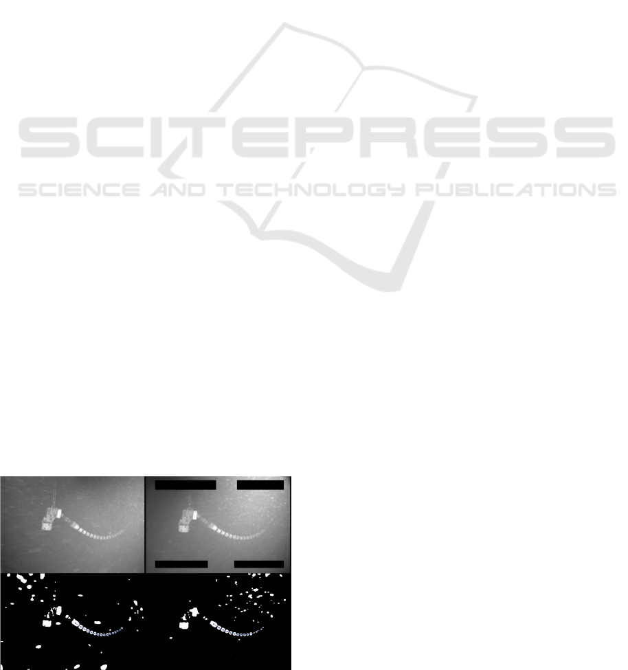
Figure 1: First row exhibits left and right images captured
by the stereo rig.
underwater environment (depth can exceed 1000m)
where the maintenance task of a flexible pipe is car-
ried out. Because of the high pressure of the environ-
ment, the task is performed by using ROVs (Remotely
Operated Vehicles) equipped with a pair of cameras.
Since no natural light can achieve such a depth, spe-
cial low light cameras are used. Despite these cameras
are sensitive to low light conditions (10
−3
LUX), they
are analog (resolution is limited to the NTSC stan-
dard) and can only capture gray scale images. In ad-
dition, the underwater environment is very noisy with
particles floating around and the pipe is almost tex-
tureless. All these characteristics lead to a final poor
quality image with limited contrast, which makes any
feature extraction almost unfeasible. In order to over-
come this problem, some high contrast markers were
previously painted over the pipe. It consists in inter-
leaved white and black regions along the pipe sur-
face. So, by using these markers a tailored solution
for the pipe segmentation was developed. This tech-
nique can provide a few stable set of features required
by the rectification technique. The tests performed so
far have shown that, at least for the presented study
case, the segmentation solution using temporal coher-
ence is robust enough to produce no outliers. How-
ever, it can be extended with RANSAC (Fischler and
Bolles, 1981) in order to ensure robustness in more
critical cases. A sample of the captured images and
the segmentation results can be seen in Fig. 1. It
worth to mention that this painting is required not
648
Cesar V., Farias T., Pessoa S., Macedo S., Kelner J. and Santos I..
Uncalibrated Image Rectification for Coplanar Stereo Cameras.
DOI: 10.5220/0004745106480655
In Proceedings of the 9th International Conference on Computer Vision Theory and Applications (VISAPP-2014), pages 648-655
ISBN: 978-989-758-009-3
Copyright
c
2014 SCITEPRESS (Science and Technology Publications, Lda.)

only by the feature extraction process, but by the sub-
sequent tracking stage that will not be approached in
this paper. Then, painting the pipe would be required
even if the rectification process would not exist. Pre-
viously calibrating the pair of cameras is something
that would be inconvenient because the cameras are
mounted during the maintenance task and the techni-
cians are not trained for it.
The current methods for rectification do not work
properly in a noisy environment with a reduced num-
ber of feature correspondences, especially when the
calibration is unknown. Thus, this paper presents a
novel rectification technique for stereo rigs that op-
erates even with a reduced number of feature cor-
respondences. The state of the art techniques (such
as (Fusiello and Irsara, 2008)) need at least six cor-
respondences, while the proposed technique requires
only three. However, the proposed solution requires
the following restrictions on the cameras rig: cam-
eras’ projection planes must be coplanar; and cameras
must have equal intrinsic parameters.
Tests were carried out in order to evaluate the
proposed technique. Three different sets of tests
were applied to measure the error related to the tech-
nique. The first one considered a synthetic test that
was proposed only with points numerically disturbed
by a random generated noise. In the second test, a
real structured environment was built and a carefully
mounted stereo rig was used.
The third test occurred in a real scenario. As stated
before, the technique was tested in a deep underwater
environment, where images were captured by a ROV.
2 RELATED WORK
Rectification of stereo images is a frequently in-
vestigated topic by the computer vision community.
These researches began by photogrammetrists, such
as (Slama et al., 1980), which were further developed
by computer vision researchers aiming to facilitate the
feature matching between images from a stereo rig.
Rectification techniques can be classified into two
categories: calibrated, and uncalibrated. Calibrated
techniques assume that cameras’ intrinsic and extrin-
sic parameters are known and the rectifying homogra-
phies are estimated only by taking into account these
parameters. In (Fusiello et al., 2000), a simple and
effective calibrated method is presented.
Uncalibrated techniques estimate the rectifying
homographies by using a set of corresponding 2D
points between the images and/or epipolar restrictions
(such as the fundamental matrix). These techniques
are more used than the calibrated ones because in
most of the real problems the rectification is required
in a stage before the cameras poses are known. How-
ever, it is a more complex problem with non-linear
solutions, which requires the use of approximations
and optimization methods. Such methods are required
because there are infinite pairs of rectifying homo-
graphies, although it is convenient to choose the one
which produces less image deformation. Some un-
calibrated techniques can be found in (Hartley, 1998),
(Loop and Zhang, 1999), (Isgro and Trucco, 1999),
(Fusiello and Irsara, 2008).
When the epipole is close to or inside the image,
image deformation tends to be large. In these cases
planar rectifications are not enough, therefore it is
necessary to use different techniques such as cylin-
drical rectification (Roy et al., 1997) or polar rectifi-
cation (Pollefeys et al., 1999).
In the scenario presented by this paper only part of
cameras parameters are previously known, which en-
forces the use of an uncalibrated technique. However,
uncalibrated techniques require at least six accurate
corresponding points between the images (Fusiello
and Irsara, 2008), requirement that may not always
be fulfilled by the application. The proposed tech-
nique overcomes this limitation by relying on some
restrictions imposed on the stereo rig. In practice,
these constrain the way in which cameras must be
relatively positioned and oriented. If the stereo rig
is mounted so that the cameras’ projection planes are
coplanar, epipoles will be localized close to the infin-
ity, enabling a planar rectification to solve the prob-
lem.
3 BACKGROUND
In this section, some concepts that are at the core of
the proposed rectification technique will be presented
as well as the adopted notation. These concepts are
more extensively explained in (Hartley and Zisser-
man, 2004), (Loop and Zhang, 1999).
3.1 Epipolar Geometry
Given two pinhole cameras P and P
0
with their re-
spective projection matrices defined as P = K[I|0] and
P
0
= K
0
R[I|−C]. I is a 3 × 3 identity matrix. Camera
P has its projection center at the origin of the coordi-
nate system 0 = [0, 0, 0]
>
. Camera P
0
has its projec-
tion center at C = [x
c
, y
c
, z
c
]
>
, defined in Euclidean
coordinates. Furthermore, matrices K and K
0
are the so
called calibration matrices, which encapsulate cam-
eras’ intrinsic parameters. A simplified calibration
matrix has the form diag( f , f , 1), where f is the lens
UncalibratedImageRectificationforCoplanarStereoCameras
649

focal length. This simplified form assumes that the
principal point is the center of the image where the
pixel skew is zero and the pixel aspect ratio is one.
The canonical form of the cameras matrices P and
P
0
are calculated aplying a projective transformation
to the 3D space such that P = [I|0].
Given a 3D point X in homogeneous coordinates,
its projection in image I through camera P is given
by x = PX. Likewise, x
0
= P
0
X is the projection of X
in image I
0
through the camera P
0
.
By using these projected points, the epipolar con-
straint can be established as
x
0>
Fx = 0, (1)
which is valid for all 2D point correspondences x ↔
x
0
. F is a 3 × 3 rank 2 matrix named fundamental ma-
trix, which maps points from image I to lines (named
epipolar lines) in image I
0
. Given the line l
0
= Fx
in image I
0
, it can be said that x
0
lies on l
0
since
x
0>
l
0
= 0. The reverse idea is also valid, and therefore
point x lies on the line l = F
>
x
0
. All epipolar lines
of one image intersect each other at a single point
named epipole, where e is the epipole in I and e
0
is
the epipole in I
0
.
Being P
can
and P
0
can
two projection matrices from
canonical cameras, i.e. P
can
= [I|0] and P
0
can
=
P
0
H
can
= [M|m], the fundamental matrix between the
two images captured by these cameras can be defined
as
F = [m]
×
M, (2)
where [m]
×
stands for the antisymmetric matrix that
is equivalent to the cross product with m.
Two images
¯
I and
¯
I
0
are said to be rectified if all
matching points
¯
x = [ ¯x, ¯y, 1]
>
and
¯
x
0
= [ ¯x
0
, ¯y
0
, 1]
>
have
the same coordinate in y, i.e. ¯y = ¯y
0
. Thus, with the
rectified matching points on the same line, the stereo
matching is made easier and computationally faster.
The rectifying process consists in estimating two
homographies H and H
0
, which when applied to im-
ages I and I
0
, respectively, make them rectified.
The epipolar geometry between two rectified im-
ages has some noteworthy particularities. The fun-
damental matrix between two rectified images is
¯
F =
[[1, 0, 0]
>
]
×
All the epipolar lines of a rectified image are par-
allel to the x direction of the image, since
¯
l
0
=
¯
F
¯
x =
[0, 1, − ¯y]
>
. Assuming all epipolar lines intersect at
the epipoles, the epipoles are valued [1, 0, 0]
>
.
3.2 Loop and Zhang Algorithm
Loop and Zhang in (Loop and Zhang, 1999) present
a rectification algorithm that uses the epipolar restric-
tions of the images. This algorithm aims to rectify
images by minimizing the distortion caused by pro-
jective transformations. The algorithm requires the
fundamental matrix and the epipole in the first image.
The strategy adopted by the algorithm is to de-
compose the rectifying homographies in three trans-
formation: 1) a projective transformation H
p
, that
maps the epipoles to the infinity; 2) a similarity trans-
formation H
r
, that rotates and translates the epipoles
to [1, 0, 0]
>
; and 3) a shearing transformation H
s
that
minimizes image distortion in the x coordinates. Us-
ing the notation defined in Section 3.1, the transfor-
mations H and H
0
, which rectify the images I and I
0
respectively, are defined as
H = H
s
H
r
H
p
(3)
and
H
0
= H
0
s
H
0
r
H
0
p
. (4)
To compute the projective transformation, two
lines must be defined: w = [w
1
, w
2
, w
3
]
>
and w
0
=
[w
0
1
, w
0
2
, w
0
3
]
>
. The lines w and w
0
pass through
epipoles e and e
0
, respectively. In order to map the
epipoles to infinity, one has to define projective the
transformations H
p
and H
0
p
that respectively map w
and w
0
to infinity. Since there are an infinity number
of possible lines, it is preferred to choose the ones that
minimize image distortions. Therefore, the projective
transformations are defined as
H
p
=
1 0 0
0 1 0
w
1
w
2
w
3
. (5)
Similarly we can define H
0
p
.
After projective transformations, epipolar lines
become parallel one another considering the same im-
age, although they are not aligned considering the
matching lines between the images. The similarity
transformations rotate and translate images in order
to make the epipolar lines parallel to the x direction.
These transformations are
H
r
=
F
32
− w
2
F
33
w
1
F
33
− F
31
0
F
31
− w
1
F
33
F
32
− w
2
F
33
F
33
+ v
0
c
0 0 1
(6)
and
H
0
r
=
w
0
2
F
33
− F
23
F
13
− w
0
1
F
33
0
w
0
1
F
33
− F
13
w
0
2
F
33
− F
23
v
0
c
0 0 1
, (7)
where v
0
c
is a common vertical translation for both im-
ages.
The homographies H
r
H
p
and H
0
r
H
0
p
are already able
to rectify the images, although shearing transforma-
tions can be added in order to minimize images distor-
tion. This transformation only modify x coordinates,
without affecting the rectification. In short, it is sim-
ply an attempt to preserve perpendicularity and aspect
ratio of the images.
VISAPP2014-InternationalConferenceonComputerVisionTheoryandApplications
650

4 METHODOLOGY
The following methodology draws its actions from
the constraints aforementioned, where the cameras
have coplanar projection planes and the identical in-
trinsic parameters. Since camera P is at the origin,
its projection matrix can be expressed as P = K[I|0],
where K is the calibration matrix (intrinsic parame-
ters). Matrix K is stated as diag( f , f , 1), where f is
the lens focal length. Camera P
0
has a translation
along the xy plane and a rotation by θ around its opti-
cal axis. In addition, camera P
0
has the same intrinsic
calibration of camera P . Thus, the projection matrix
of camera P
0
is defined as P
0
= KR[I|−C], where R is
a tridimensional counterclockwise rotation by angle
θ about z axis and C = [x
c
, y
c
, 0]
>
. In order to sim-
plify further calculations, C vector will be presented
as C = d[cosα, sin α, 0], with d = ||C||.
To obtain the canonical form of the camera matri-
ces, we can define the transformation
H
can
=
K
−1
0
0
>
1
, (8)
resulting in P
can
= [I|0] and P
0
can
= P
0
H
can
=
[KRK
−1
| − RC] = [R| − RC]. By using these matrices
and (2) one can calculate the fundamental matrix re-
lated to P and P
0
, resulting in
F = [−RC]
×
R
= −d
0 0 sin(α + θ)
0 0 −cos(α + θ)
−sin α cosα 0
.
(9)
Once the fundamental matrix is up to scale, factor
−d can then be removed from (9). The epipoles from
F and F
>
are extracted using the nullspace of these
matrices, giving respectively
e = null(F) = [cotα, 1, 0]
>
(10)
and
e
0
= null(F
0
) = [cot(α + θ), 1, 0]
>
.
(11)
After calculating the epipolar geometry, the rec-
tifying homographies can be found by applying the
Loop and Zhang’s algorithm (Loop and Zhang, 1999).
The first step is to define the projective transfor-
mations that map epipoles to infinity. In order to de-
fine these transformations, one has to determine the
lines w and w
0
.
As stated in (10) and (11), epipoles are already at
infinity if cameras are coplanar, so the line at infinity
l
∞
= [0, 0, 1]
>
must be chosen in order to avoid image
distortion. Then
w = w
0
= [0, 0, 1]
>
, (12)
which, by (5), leads to H
p
= H
0
p
= I.
The following step maps, through a rotation and
translation, the epipoles onto the point [1, 0, 0]
>
. In
(Loop and Zhang, 1999), the mapping is given by (6)
and (7), which depends on F, w, and w
0
. Using (9)
and (12) to fill (6) and (7), one can get
H
r
=
cosα sin α 0
−sin α cosα 0
0 0 1
(13)
and
H
0
r
=
cos(θ + α) sin(θ + α) 0
−sin(θ + α) cos(θ + α) 0
0 0 1
. (14)
The last step of Loop and Zhang’s algorithm deter-
mines affine transformations in order to preserve the
aspect ratio and perpendicularity of image. It is also
worth to mention that H
p
H
r
and H
0
p
H
0
r
are rigid trans-
formations, therefore this step is not necessary. So,
one can define H
s
= H
0
s
= I.
By using the rectifying homographies calculated
as (3) and (4), the proposed method, adapted from
Loop and Zhang’s technique for cameras with copla-
nar projection planes can be summarized as follows.
Given two images I and I
0
and 2D matching points
x ↔ x
0
, where x is in I and x
0
is in I
0
, the rectification
of I and I
0
consists in calculating the angle α, an-
gle β = α + θ and matches
¯
x ↔
¯
x
0
, where
¯
x = R(α)x,
¯
x
0
= R(β)x
0
, and R(θ) is a matrix representing a 2D
clockwise rotation by angle θ.
According Loop and Zhang in (Loop and Zhang,
1999), the rectification is done from the fundamental
matrix, although one can define another approach us-
ing 2D point matches to determine angles α and β.
Given
¯
x =
¯x
¯y
=
x cos α − ysinα
x sin α + ycosα
(15)
and
¯
x
0
=
¯x
0
¯y
0
=
x
0
cosβ − y
0
sinβ
x
0
sinβ + y
0
cosβ
, (16)
and knowing that the rectified image obeys constraint
¯y = ¯y
0
, one can have
x sin α + ycosα − x
0
sinβ − y
0
cosβ = 0. (17)
If there are n 2D matching points, there will be n
equations like (17), which leads to the system
x
1
y
1
−x
0
1
−y
0
1
x
2
y
2
−x
0
2
−y
0
2
.
.
.
.
.
.
.
.
.
.
.
.
x
n
y
n
−x
0
n
−y
0
n
sinα
cosα
sinβ
cosβ
= Ay = 0, (18)
where 0 is a column n-vector of zeros.
UncalibratedImageRectificationforCoplanarStereoCameras
651

The solution has two degrees of freedom and can
be reached by using only 2D matches between the two
images. The degrees of freedom are the two angles
that rotate the respective images. The aforementioned
system is non-linear due to sine and cosine functions,
and a linear approximation is not suited for a noisy
scenario.
The solution of the problem given in (18) can be
found by using two different methods that will be de-
scribed in the next subsections.
4.1 Linear Solution
This approach uses a technique called “linearization”
that was employed by (Ansar and Daniilidis, 2003)
and (Lepetit et al., 2009) to estimate pose of cameras
based on correspondences between 2D and 3D points.
This technique modifies the presentation of the prob-
lem to apply a linear approximation that satisfies its
non-linear constraints.
In order to make the problem linear, one can
substitute the non-linear part of the problem by new
variables, giving y = [sinα, cos α, sin β, cosβ]
>
=
[y
1
, y
2
, y
3
, y
4
]
>
. One must ensure that the
Pythagorirean trigonometric identities
y
2
1
+ y
2
2
= 1 (19)
and
y
2
3
+ y
2
4
= 1 (20)
still hold.
In order to find the solution space of (18) one can
solve it by using a SVD decomposition A = UDV
>
.
The approximated solution is within the space defined
by the base composed of the third and fourth columns
of V, named u and v, respectively, which are related to
the smallest singular values. Since there are two vari-
ables, the solution space is two-dimensional. Thus,
the solution to y must be a linear combination of the
vectors u = (u
1
, u
2
, u
3
, u
4
) and v = (v
1
, v
2
, v
3
, v
4
), re-
sulting
y = γu + δv. (21)
By replacing (21) in (19) and (20), one can have
(γu
1
+ δv
1
)
2
+ (γu
2
+ δv
2
)
2
= 1 (22)
and
(γu
3
+ δv
3
)
2
+ (γu
4
+ δv
4
)
2
= 1, (23)
which represent two ellipses, because ∆
1
=
−2(v
1
u
2
− v
2
u
1
)
2
and ∆
2
= −2(v
3
u
4
− v
4
u
3
)
2
are always negative.
Adding up (22) and (23), one can find
u
>
uγ
2
+ u
>
vγδ + v
>
vδ
2
=
γ
2
+ δ
2
= 2,
(24)
once u and v were picked from an orthonormal ba-
sis. Conic in (24) describes a circumference whose
equation is satisfied by intersection points of ellipses
(22) and (23). In this case, there can be two or four
intersections.
The intersections of the circumference with the
two ellipses can be found by solving a fourth order
polynomial such as ax
4
+ bx
2
+ c = 0, which has two
symmetric solutions. Such polynomial can be deter-
mined by using the Sylvester resultant. The result can
be used in (24) to determine the last variable. The
symmetric solutions are realistic because the supple-
ment of an answer is also a correct answer, once im-
ages remain rectified when rotated by 180
◦
. In the
case where there are four solutions, the one that satis-
fies γ > δ must be used.
4.2 Non-linear Solution
The system given by (18) is non-linear, and thus not
suitable for a direct solution. Therefore, another ap-
proach to tackle the problem is by using numerical
methods. Finding α and β that minimize ||Ay||
2
is a
least squares problem that can be solved by the Gauss-
Newton method. The initial values of α and β, namely
α
0
and β
0
, can be assigned in two different ways: ei-
ther by using the result of the linear method described
in this paper, or by taking both values as zero. The
second choice is acceptable because the cameras are
mounted on ROVs manually attempting to enforce the
coplanar constraints.
5 RESULTS
In an attempt to evaluate the proposed technique, this
section proposes three sets of tests, which respectively
compare the approaches proposed one another with
synthetic data, compare the best approach with the
state-of-the-art technique described by Fusiello and
Irsara (Fusiello and Irsara, 2008), and show the epipo-
lar error in a real cluttered environment.
5.1 Synthetic Simulation
The simulation proposes to compare the different ap-
proaches of the suggested method to solve the homo-
geneous system given by (18) minimizing ||Ay||. A
synthetic scene was created with two cameras, P and
P
0
, with coplanar projection planes. The intrinsic cal-
ibration of the cameras were generated considering an
image size of 800 × 600 pixels and a focal length of
965.68 pixels (a horizontal field of view around 45
◦
).
VISAPP2014-InternationalConferenceonComputerVisionTheoryandApplications
652
Table 1: Synthetic simulation results with 2 pixels of Gaussian noise (Mean±std and Iterations).
6 points 12 points 20 points
α-Error β-Error Itr α-Error β-Error Itr α-Error β-Error Itr
Linear 2.81 ± 2.91 1.71 ± 1.83 – 1.88 ± 1.91 1.16 ± 1.17 – 1.45 ± 1.49 0.90 ± 0.91 –
Non-Linear 1.16 ± 2.00 0.62 ± 1.21 5.64 0.68 ± 0.56 0.37 ± 0.32 5.14 0.50 ± 0.41 0.28 ± 0.24 4.96
Linear+Non-Linear 1.11 ± 1.14 0.59 ± 0.64 4.29 0.68 ± 0.56 0.37 ± 0.32 3.83 0.50 ± 0.41 0.28 ± 0.24 3.59
Figure 2: Synthetic results varying the amount of point correspondences and Gaussian noise.
In this simulation the cameras are 90cm apart from
each other and a 3D point cloud was randomly gen-
erated inside the frustums of the cameras and away
between 3m and 6m from their baseline. These num-
bers represent the expected configuration of the real
environment where the method will be applied. The
3D points are projected by the cameras P e P
0
and
thereafter a Gaussian noise will be added to the pro-
jections to simulate the lack of precision of the track-
ing process. These projected points are the input for
the rectification method proposed in this work. The
non-linear technique will be evaluated against both
initializing α
0
and β
0
with zero values and with the
solution of the linear approach.
The results were obtained using 6, 12 and 20 3D
points. The Gaussian noise applied to the projections
has standard deviation from 0.5 to 4 pixels. For each
noise (standard deviation) generated, the tests were
computed 2000 times in order to reach an accurate
evaluation. In each sample, the values used for α and
θ came from a uniform distribution generating values
between −30
◦
and 30
◦
. The results are illustrated in
Fig. 2. Table 1 presents the numeric results.
Note that the precision is strongly related to the
number of points. It is also possible to observe
that the linear algorithm achieved the worst perfor-
mance with errors greater than 4
◦
, while the non-
linear achieved averaging errors below 2
◦
.
When the result of the linear algorithm feeds the
initial values of the non-linear algorithm, which uses
an iterative Gauss-Newton algorithm, one can observe
that the results are very similar to the ones where the
initial values are taken from zero (α
0
= 0 and β
0
= 0).
The difference between both approaches does not ex-
ceed 0.1
◦
. This occurs because the local minima do
not influence the convergence of the algorithm, except
when the amount of points is small.
In Table 1, one can verify that initializing the
Gauss-Newton algorithm with the linear approach de-
creases between 20% and 40% the number of itera-
tions. It is possible to observe as well that the conver-
gences in the non-linear approaches are different only
when it has six points.
Overall, one can conclude that an optimal solution
to the problem can be reached applying the Gauss-
Newton method, unless the amount of points is small
(around 6). In this case, by using as initial value the
output of the linear approach can produce more accu-
rate results.
All simulations were performed using MATLAB.
The hardware used in the tests was a computer with
an Intel Core i7 3960X 3.30Ghz processor and 24GB
RAM. The execution time was collected using a sim-
ulation with 20 3D points. In average, the linear ap-
proach takes around 0.15ms to finish, the non-linear
0.3ms, and the linear+non-linear also 0.3ms. The rea-
son why the two last approaches spend the same time
is because the non-linear approach performs fewer it-
erations when initialized by the linear approach result.
5.2 Controlled Environment Tests
In this test, a controlled environment is used to com-
pare the proposed approach to the state-of-the-art
technique of Fusiello and Irsara (Fusiello and Irsara,
2008). The test consists of two pictures of a chess-
board, as illustrated in Fig. 3. The camera used in
this test was a Canon T4i and the picture resolution
was set to 720 × 480 pixels. Only this resolution was
tested because it is closest one to the resolution of the
cameras attached to the ROV. The camera was posi-
tioned about 70cm away from the target. Between the
two shots, the camera was moved 20cm rightward and
4cm upward keeping the same focal length and en-
UncalibratedImageRectificationforCoplanarStereoCameras
653
Figure 3: Images used for the controlled environment tests.
forcing coplanarity constraint of cameras. The cam-
era was intentionally moved without an accurate pro-
cess (actually it was manually moved), while keeping
the optical axes nearly parallel. Also, the images were
manually defocused to simulate the blur phenomenon
that occurs underwater.
Since the exact position of camera is unknown,
there is no ground truth. Thus, the technique will be
evaluated using the rectification error (i.e. epipolar er-
ror, or the distance of the point to the related epipolar
line, which can be calculated as Ay). The chessboard
has 54 points that can be extracted and matched be-
tween the images. To apply the rectification, a sub-
set ranging from 6 to 20 points chosen randomly will
be used as input, although all 54 points are used to
measure the epipolar error. It is expected that the
more precise the rectification the smaller will be the
errors. For each amount of points, 100 subsets of ran-
dom points were chosen to be rectified with the non-
linear approach proposed (initialized with the linear
approach) and later with the technique proposed by
Fusiello and Irsara (Fusiello and Irsara, 2008).
In Fig. 4, it can be seen that the Fusiello and Ir-
sara’s technique had poor results with a small amount
of points, since such technique has more degrees of
freedom to be determined. However, from 12 points
on, the Fusiello and Irsara’s technique can estimate
more precisely all the system variables than the pro-
posed technique.
In Fig. 5 the rectification of the left image using
6 points is shown. The rectification from Fusiello and
Irsara applied more distortion to the images and has
a strong projective distortion, as well. Such result is
not acceptable as the epipoles are close to the infinity.
As expected, the proposed technique applied a simple
rotation.
The tests were carried out using the same hard-
ware from the synthetic simulation. The proposed
technique, due to its complex minimization calcula-
tions, had an execution time between 0.2 and 0.3ms.
Fusiello and Irsara’s technique had an average time of
230ms with 6 points and 3s with 20 points.
5.3 Real Experiments
This work was also tested with real underwater im-
Figure 4: Comparison of the results obtained with Fig. 3 by
the proposed technique and the Fusiello and Irsara’s tech-
nique.
(a) (b)
Figure 5: Rectification of the left image of Fig. 3 using (a)
the proposed technique and (b) Fusiello and Irsara’s tech-
nique.
ages. The cameras used for the operations were
Kongsberg OE15-100c (low light cameras for high
depths). These cameras are attached to the ROV by a
metal support and are 45cm apart. The support of the
cameras is an attempt to keep the cameras’ projection
planes parallel. The system first segments the flexible
pipe from both left and right images in order to ex-
tract features. The segmentation is performed in two
stages: first, a tailored thresholding technique is used
to find out which regions are potentially of the pipe
(the white blobs in the second row of Fig. 1); second,
a search is performed in order to discover the best se-
quence of thresholded regions which describe a pipe.
Since the features are extracted by evaluating the cen-
troid of the thresholded regions, features position are
not very precise. These features are then matched be-
tween both images. The amount of extracted features
ranges from 5 to 16. Even without a groundtruth, the
achieved results can testify the technique efficiency.
Fusiello and Irsara’s technique was also tested
with the real underwater images. However, it fails in
many cases because the estimated homographies pro-
duce huge projective distortions, while only a rotation
and a small projective transformation are needed (as
illustrated in Fig. 6(a)). In addition, consecutive pairs
of images (i.e., similar images) produced completely
different homographies, which is mostly due to inac-
curacies in the detection of features position. In Fig.
VISAPP2014-InternationalConferenceonComputerVisionTheoryandApplications
654
(a)
(b)
Figure 6: Rectification of the images of Fig. 1 using (a)
Fusiello and Irsara’s and (b) the proposed technique.
6(a) the red circle shows that this part of the image is
not correctly rectified.
The proposed technique achieved better results
than the Fusiello and Irsara’s technique. The results
along multiple frames were also more stable. The ro-
tation angle in the first image was between 9
◦
and 13
◦
while the second image was between 10
◦
and 14
◦
.
The epipolar error ranges from 0.5 to 1.2 pixels. Fig.
6(b) illustrate the result. The red circle shows that, in
contrast with the Fusiello and Irsara’s technique, this
part of the image is correctly rectified.
After the initial rectification, the images were
aligned allowing the extraction of more information
about the visual landmarks in order to perform a more
accurate 3D reconstruction. Thus, the error embedded
in the rectification process is acceptable for the whole
system. Outliers were not detected in the tests, how-
ever they could be removed using RANSAC-based al-
gorithms.
6 CONCLUSIONS
This paper proposed a novel rectifying technique
for images under constraints imposed by underwater
maintenance tasks. The proposed technique takes ad-
vantage of the geometry of the structure of the stereo
rig, which is positioned keeping the cameras’ pro-
jection planes coplanar. This arrangement represents
lesser degrees of freedom for the rectification prob-
lem, which allows lesser point correspondences to ob-
tain satisfactory accuracy, as well.
Tests were carried out using synthetic data, a real
controlled environment and a real underwater scene.
The proposed technique performed better than the
state-of-the-art method (Fusiello and Irsara, 2008).
As future work, the present technique will be im-
proved to take into consideration variations on the in-
trinsic parameters of the cameras, such as focal length
and principal point, which were considered to be fixed
under the performed tests.
REFERENCES
Ansar, A. and Daniilidis, K. (2003). Linear pose estimation
from points or lines. IEEE Transactions on Pattern
Analysis and Machine Intelligence, 25:282–296.
Fischler, M. A. and Bolles, R. C. (1981). Random sample
consensus: a paradigm for model fitting with appli-
cations to image analysis and automated cartography.
Commun. ACM, 24(6):381–395.
Fusiello, A. and Irsara, L. (2008). Quasi-euclidean uncal-
ibrated epipolar rectification. In Pattern Recognition,
2008. ICPR 2008. 19th International Conference on,
pages 1–4.
Fusiello, A., Trucco, E., and Verri, A. (2000). A compact al-
gorithm for rectification of stereo pairs. Mach. Vision
Appl., 12(1):16–22.
Hartley, R. I. (1998). Theory and practice of projective rec-
tification.
Hartley, R. I. and Zisserman, A. (2004). Multiple View Ge-
ometry in Computer Vision. Cambridge University
Press, ISBN: 0521540518, second edition.
Isgro, F. and Trucco, E. (1999). Projective rectification
without epipolar geometry. In Computer Vision and
Pattern Recognition, 1999. IEEE Computer Society
Conference on., volume 1, pages –99 Vol. 1.
Lepetit, V., Moreno-Noguer, F., and Fua, P. (2009). Epnp:
An accurate o(n) solution to the pnp problem. Int. J.
Comput. Vision, 81(2):155–166.
Loop, C. and Zhang, Z. (1999). Computing rectify-
ing homographies for stereo vision. In Computer
Vision and Pattern Recognition, 1999. IEEE Com-
puter Society Conference on., volume 1, pages 2 vol.
(xxiii+637+663).
Pollefeys, M., Koch, R., and Van Gool, L. (1999). A sim-
ple and efficient rectification method for general mo-
tion. In Computer Vision, 1999. The Proceedings of
the Seventh IEEE International Conference on, vol-
ume 1, pages 496 –501 vol.1.
Roy, S., Meunier, J., and Cox, I. (1997). Cylindrical recti-
fication to minimize epipolar distortion. In Computer
Vision and Pattern Recognition, 1997. Proceedings.,
1997 IEEE Computer Society Conference on, pages
393 –399.
Slama, C. C., Theurer, C., and Henriksen, S. W., editors
(1980). Manual of Photogrammetry. American Soci-
ety of Photogrammetry.
UncalibratedImageRectificationforCoplanarStereoCameras
655
