
Observer Design for a Nonlinear Minimal Model of Glucose
Disappearance and Insulin Kinetics
Driss Boutat
1
, Mohamed Darouach
2
and Holger Voos
3
1
INSA Centre Val de Loire, Univ. Orl´eans, PRISME EA 4229, 88 boulevard Lahitolle 18020, Bourges cedex, France
2
CRAN-CNRS, UHP Nancy I, IUT de Longwy 186, rue de Lorraine, 54400 Cosnes-et-Romain, France
3
Universit´e du Luxembourg, Facult´e des Sciences, de la Technologie et de la Communication,
6, rue Richard Coudenhove-Kalergi, L-1359, Walferdange, Luxembourg
Keywords:
Nonlinear Dynamical Systems, Observer Design, Insulin Kinetics.
Abstract:
This work deals with an observer design for a nonlinear minimal dynamic model of glucose disappearance
and insulin kinetics (GD-IK). At first, the model is transformed into a nonlinear observer normal form. Then,
using the knowledge of the plasma blood glucose level, we estimate the state variables that are not directly
available from the system, i.e. the remote compartment insulin utilization, the plasma insulin deviation and
the infusion rate. In addition, we estimate the amount of absorbed glucose by means of the inverse dynamics.
1 INTRODUCTION
Diabetes is a serious disease by which the body’s pro-
duction and use of insulin are impaired, causing an
increase of glucose concentration level in the blood-
stream. Regulating blood glucose levels as close to
normal as possible leads to a substantial decrease in
long term complications of diabetes. The most com-
mon treatment of diabetes type 1 (where the insulin
production of the pancreas is disturbed) is the mea-
surement of the glucose level using suitable measure-
ment devices to regulate this level with an injection
of insulin. Advanced solutions are trying to apply au-
tomatic feedback control for this process using glu-
cose level sensors and insulin infusion pumps, see
e.g. (Chee et al., 2003) for a comprehensive overview
of the technological aspects. But all currently avail-
able solutions are far from being optimal. One main
problem is the fact that not all important variables are
known or measurable. Therefore, observers play a
very important role in this control task and will also
be the main issue of this contribution.
First of all the development of suitable observers
as well as control algorithms requires the derivation
of a dynamic mathematical model of the system un-
der control, i.e. the complex dynamics of glucose dis-
appearance and insulin kinetics(GD-IK). During the
last decades, considerable research has been devoted
to the derivation and improvement of such models,
and many of them have already been described in
the literature ranging from simple expressions to very
complex nonlinear mathematical models (Chee et al.,
2003). One model which is commonly used in the
literature is the so called minimal model. It is a sin-
gle input-output nonlinear dynamic system with four
states: the plasma insulin concentration level i(t), the
plasma blood glucose level g(t), a variable v(t) which
is proportional to the insulin in the remote compart-
ment and w(t) which represents the infusion rate by
means of a pump. The input variable of this minimal
GD-IK modelis the effect of a pump while the plasma
blood glucose level is the output.
Most research which is so far interested in control
or observer synthesisusing the minimal GD-IK model
is based on linearization of this model, see (Percival
et al., 2008), (Magni et al., 2007), (Hariri and Wang,
2011), (Gonz´alez and Femat, 2011), (Parker et al.,
1999), (Bergman et al., 1979), (L Kovcs, 2007) and
references therein. More recent work on the same
theme can be found in (Eberle and Ament, 2012) and
(Villafaa-Rojas et al., 2013). In this paper however,
we will design an observer for the nonlinear minimal
GD-IK model without any simplification. Indeed, we
will transform this model into a nonlinear observer
normal form. The considered model also contains an
unknown amount g
M
of glucose absorption from the
gut which will be estimated by the dynamic inversion
method. Furthermore, we distinguish two situations
in this work: the case where g
M
is known and the case
where g
M
is considered as an unknown disturbance
21
Boutat D., Darouach M. and Voos H..
Observer Design for a Nonlinear Minimal Model of Glucose Disappearance and Insulin Kinetics.
DOI: 10.5220/0004747700210026
In Proceedings of the International Conference on Bio-inspired Systems and Signal Processing (BIOSIGNALS-2014), pages 21-26
ISBN: 978-989-758-011-6
Copyright
c
2014 SCITEPRESS (Science and Technology Publications, Lda.)

rate. On the one hand, our contribution is based on
the works of (Krener and Isidori, 1983), (Respondek
and Pogromsky, 2004), (Boutat, 2007), (Boutat and
Busawon, 2011), (Boutat et al., 2009) in order to de-
rive a change of coordinates that transforms the mini-
mal GD-IK model into an observer nonlinear normal
from. This enables us to design a robust observer.
On the other hand, it is based on works of (Kudva
et al., 1980), (Yang and Wilde, 1988), (Darouach
et al., 1994), (Hui and Zak, 2005), (Bhattacharyya,
1978) to build an observer based on unknown distur-
bances.
This paper is organized as follows. The next sec-
tion presents the nonlinear minimalGD-IK modeland
states the problem to be solved. The third section
deals with the change of coordinatesand describes the
observer nonlinear normal form. The fourth section is
devoted to the design of two types of observers, a full
order observer by assuming that g
M
is known and a
reduced observer in the case where g
M
is unknown.
2 NOTATIONS AND PROBLEM
STATEMENT
In this paper the considered nonlinear minimal GD-
IK model is a combination of models extracted from
papers of (Hariri and Wang, 2011), (Percival et al.,
2008):
˙g = −P
1
g(t) − g(t)v(t) + P
1
g
b
+ g
M
(t)
˙v = −P
2
v(t) + P
3
i(t) − P
3
i
b
˙
i = −ni(t) + γ(g(t) − h)t
y = g(t)
(1)
where g(t) is the plasma blood glucose level; i(t) is
the plasma insulin concentration level; v(t) is the vari-
able which is proportional to the insulin in the remote
compartment, g
b
is the basal blood glucose level, g
M
is the rate of glucose absorption from meal (glucose
absorption from the gut) and i
b
is the basal insulin
level. Parameter P
1
represents glucose effectiveness,
P
2
denotes the decreasing level of insulin, P
3
is the
rate at which insulin action is increased as the level
of insulin deviates from the corresponding baseline, γ
is the rate at which insulin is produced, n denotes the
fractional insulin clearance and h denotes the pancre-
atic target glycemia level. As in ((Hariri and Wang,
2011)), we add to the above model the pump dynam-
ics:
˙w =
1
a
(−w(t) + u(t)) (2)
where w(t) represents the infusion rate, u(t) the con-
trol input and a denotes the time constant of the
pump. From now on, this model is rewritten in a
general state variable format with four state variables
x
1
(t) = g(t), x
2
(t) = v(t), x
3
(t) = i(t), x
4
(t) = w(t):
˙x
1
= −P
1
x
1
− x
1
x
2
+ P
1
g
b
+ g
M
(t)
˙x
2
= −P
2
x
2
+ P
3
x
3
− P
3
i
b
˙x
3
= −nx
3
+ x
4
+ γ(x
1
− h)t
˙x
4
= −
1
a
x
4
+
1
a
u
y = x
1
(3)
This dynamic system can be further expressed in the
following compact form:
˙x = f(x) + B
1
u+ ν(t,y) + g
M
(t)B
2
y = h(x)
(4)
where
• x = (x
1
,x
2
,x
3
,x
4
)
T
is the vector of state variables
and h(x) = x
1
is the output,
• f(x) =
−x
1
x
2
,−P
2
x
2
+ P
3
x
3
,−nx
3
+ x
4
,−
1
a
x
4
T
is the drift vector field
• B
1
=
0,0,0,
1
a
T
is the control direction,
• B
2
=
1,0,0, 0
T
is the unknown direction,
• ν(t,y) =
P
1
g
b
− P
1
y,−P
3
i
b
,γ(y− h)t, 0
T
is a
direction depending on the output y and time t.
In this work, we consider the following problem:
How can we find a change of coordinates z = φ(x) in
order to transform (3) into a nonlinear observer nor-
mal form, i.e.
˙z = A
O
z+ β(y,t) +
B
1
u+ α(y)g
M
(t)
y = C
O
z = z
4
(5)
where A
O
=
0 0 0 0
1 0 0 0
0 1 0 0
0 0 1 0
, C
O
=
0 0 0 1
, and the new output
y = ϕ(y)
is a diffeomorphism of the output y. In addition, this
nonlinear observer normal form enables us to deal
with the following problems: (i) Design an observer-
based feedback if g
M
(t) is known or if g
M
(t) = 0
and (ii) Design an observer-based feedback by the
concept of inversion dynamics if g
M
(t) is unknown.
3 NONLINEAR OBSERVER
NORMAL FORM OF GD-IK
3.1 Transformation Algorithm
There are several sophisticated geometrical algo-
rithms that enable us to transform the dynamic sys-
tem (4) into a nonlinear observer normal form (5), see
BIOSIGNALS2014-InternationalConferenceonBio-inspiredSystemsandSignalProcessing
22

(Krener and Isidori, 1983), (Respondek and Pogrom-
sky, 2004), (Boutat, 2007), (Boutat and Busawon,
2011). In this paper, thanks to the special form of
the proposed system, we can establish an algorithm
based on matrix calculus. At the same time, we pro-
vide an algorithm to compute change of coordinates.
For this purpose, let us consider a single input-output
dynamic system with the following form:
˙x = Ax+ µ(y,t, u,s(t))
y = Cx
(6)
with the vector of state variables x ∈ R
n
, the output
y ∈ R and the function µ(y,t, u,s(t)) which does not
depend on the unmeasured state. We assume that the
pair (C,A) is observable. Thus, the matrix
O =
C
CA
...
CA
n−1
is of full rank n. Let p(s) = s
n
+ a
n−1
s
n−1
+
a
n−2
s
n−2
+ ... + a
1
s + a
0
be the characteristic poly-
nomial of the matrix A. We recall that the Cayley-
Hamilton theorem states that p(A) = 0. Then the fol-
lowing result holds.
Theorem 1. The following linear change of coordi-
nates
z
n
= Cx
z
n−i
= CA
i
x+
∑
i
k=1
a
n−k
CA
i−k
x for i = 1 : n− 1
(7)
transforms the dynamic system (6) into the following
observer normal form:
˙z = A
O
z+
µ(y,t,u,v(t))
y = C
O
z = z
n
(8)
where the pair (C
O
,A
O
) is in Brunovsky canonical
form and
µ is defined by its components as follows
µ
n
= Cµ− a
n−1
y
µ
n−i
= CA
i
µ+
∑
i
k=1
a
n−k
CA
i−k
µ− a
n−i−1
y
for i = 1 : n− 1
(9)
Proof. We proceed by successive derivation of the
change of coordinates given in (7). Then, we obtain:
˙z
n
= CAx +Cµ = z
n−1
− a
n−1
y+Cµ
˙z
n−i
= z
n−i−1
− a
n−i−1
y+CA
i
µ+
+
i
∑
k=1
a
n−k
CA
i−k
µ (10)
for i = 1 : n − 2 (11)
˙z
1
= −a
0
y+CA
n−1
µ+
n−1
∑
k=1
a
n−k
CA
n−1−k
µ
where the last equation is obtained by using the
Cayley-Hamilton theorem.
3.2 Application to the GD-IK
In this subsection, we will apply the results obtained
in the previous section to the GD-IK model. Let us
consider the nonlinear dynamic system (3). We start
by transforming it first into the form (6). For this we
use the concept of diffeomorphism on the output (see
(Respondek and Pogromsky, 2004) ,(Boutat, 2007),
(Boutat and Busawon, 2011), (Boutat et al., 2009)). In
our case we define the new output
y = − ln(y). Hence,
if we consider the new variable ξ = − ln(x
1
), then the
dynamic system (3) is rewritten as follows:
˙
ξ = x
2
+ P
1
− P
1
e
y
g
b
− e
y
g
M
˙x
2
= −P
2
x
2
+ P
3
x
3
− P
3
i
b
˙x
3
= −nx
3
+ x
4
+ γ(e
−
y
− h)t
˙x
4
= −
1
a
x
4
+
1
a
u
y = ξ = − lny
(12)
With the definition of the matrix
A =
0 1 0 0
0 −P
2
P
3
0
0 0 −n 1
0 0 0 −
1
a
and the vector C =
1 0 0 0
, the dynamic
system givenin (12)can be written in the desired form
given in (6):
˙
X = AX + B
1
u+ B
2
(y)g
M
+ β(y,t)
y = CX = ξ
with X = (ξ, x
2
,x
3
,x
4
)
T
and µ = B
1
u + B
2
(
y)g
M
+
β(y,t).
As the pair (C,A) is observable, we can use Theo-
rem 1. The characteristic polynomial of A is given by
s
4
+
n+ P
2
+
1
a
s
3
+
1
a
(n+ P
2
) + nP
2
s
2
+
1
a
nP
2
s,
then the change of coordinates can be given by th fol-
lowing expression:
z
1
=
1
a
P
3
x
3
+
n
a
x
2
+ P
3
x
4
−
1
a
nP
2
lnx
1
z
2
= P
3
x
3
+
n+
1
a
x
2
−
1
a
(n+ P
2
) + nP
2
lnx
1
z
3
= x
2
+
n+ P
2
+
1
a
lnx
1
z
4
= − lnx
1
= ξ
Therefore, we obtain the nonlinear observer normal
form (6) for the nonlinear dynamic system (3) as fol-
lows:
˙z = A
O
z+ β(y,t) +
B
1
u+ α(y)g
M
(t)
y = C
O
z = z
4
(13)
where
• β(
y,t) =
β
1
,β
2
,β
3
,β
4
T
with
β
1
=
1
a
e
−
y
− h
tγP
3
−
1
a
nP
3
i
b
+
1
a
nP
2
P
1
+
P
1
y
1
a
nP
2
g
b
, β
2
=
1
a
nP
2
lnx
1
+
ObserverDesignforaNonlinearMinimalModelofGlucoseDisappearanceandInsulinKinetics
23
P
3
γ(e
−y
− h)t −
n+
1
a
P
3
i
b
+
1
a
(n+ P
2
) + nP
2
P
1
+
P
1
y
(
1
a
(n+ P
2
) + nP
2
)g
b
,
β
3
= −
1
a
(n+ P
2
) + nP
2
y − P
3
i
b
+
n+ P
2
+
1
a
P
1
+
P
1
y
(n + P
2
+
1
a
)g
b
,
β
4
= −
n+ P
2
+
1
a
y+ P
1
+
P
1
y
g
b
•
B
1
=
P
3
a
,0,0,0
T
• α(
y) =
1
y
1
a
nP
2
,
1
a
(n+ P
2
) + nP
2
,n+ P
2
+
1
a
,1
T
4 OBSERVER DESIGN
In this section we will present two types of observers.
The first one assumes that g
M
is known and the second
one assumes that g
M
is unknown. In the last case we
will design an observer to estimate both the state and
g
M
. First, it should be noted that (13) is controllable.
4.1 Full Order Observer
In the first case, we consider (13) and we define the
following observer-based feedback:
˙
ˆz = A
O
ˆz+ β(y,t) +
B
1
u+ α(y)g
M
+ K(
ˆ
y− y). (14)
If we set the observation error e = ˆz − z, we can
obtain that its dynamics is linear and given by ˙e =
(A
O
+ KC
O
)e.As the pair (C
O
,A
O
) is observable we
can find a gain K such that A
O
+ KC
O
is asymptoti-
cally stable.
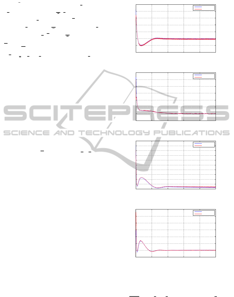
We provide also an observer-based feedback with
u = Kˆz such that the output g(t), the glucose level,
reaches the glucose basal level (99mg/dl) , see also
Fig. 1. The estimations of the states as well as the
actual values obtained in the simulation are given in
Fig. 2 - Fig. 4, respectively. The parameters and ini-
tial states used in the simulations are: P
1
= 0 P
2
=
0.81/100, P
3
= 4.01/1e6 n = 0.23, a = 2, gb =
99, ib = 8 , γ = 2.4/1000, h = 93 , x
1
(0) =
337 , x
2
(0) = 0, x
3
(0) = 192 , x
4
(0) = 2. These pa-
rameters and initial states are the same as in (Hariri
and Wang, 2011).
4.2 Observer for Unknown Input
In the second case we assume that g
M
is an unknown
input and we will design an observer to estimate both
the state and g
M
. If we consider g
M
as an unknown
input, we can follow (Kudva et al., 1980), (Yang and
Wilde, 1988), (Darouach et al., 1994), (Hui and Zak,
2005), (Bhattacharyya, 1978) which leads to a de-
composition of the state of the observer normal form
(13) into two parts, namely the unmeasurable and the
0 200 400 600 800 1000
80
90
100
110
120
130
140
150
g(t)
Times [s]
g(t)
estimation
Figure 1: Evolution of g(t).
0 200 400 600 800 1000
−2
0
2
4
6
8
10
12
x 10
−3
v(t)
Times [s]
v(t)
estimation
Figure 2: Evolution of v(t).
0 200 400 600 800 1000
0
20
40
60
80
100
120
140
160
180
200
i(t)
Times [s]
i(t)
estimation
Figure 3: Evolution of i(t).
0 200 400 600 800 1000
0
2
4
6
8
10
12
14
w(t)
Times [s]
w(t)
estimation
Figure 4: Evolution of w(t).
measurable part: z = (I − MC)z + MCz = q + My,
where
M =
1
C
O
α
α =
1
a
nP
2
,
1
a
(n+ P
2
) + nP
2
,n+ P
2
+
1
a
,1
T
is a constant matrix even if α is not constant. There-
fore we have the following projector:
BIOSIGNALS2014-InternationalConferenceonBio-inspiredSystemsandSignalProcessing
24

˜
Π = I − MC =
1 0 0 −
1
a
nP
2
0 1 0 −
1
a
(n+ P
2
) + nP
2
0 0 1 −
n+ P
2
+
1
a
0 0 0 0
.
Now, we consider the dynamics of the unknown part
q. Thanks to the fact that
˜
Πα = 0, we obtain ˙q =
˜
Π
A
O
q− My+
B
1
u+ β(y,t)
. An observer for this
last dynamic system is derived as follows:
˙
bq =
˜
Π
A
O
bq− My+
B
1
u+ β(y,t)
−
−
˜
Π(LC
O
(bq− q)) (15)
bz = bq+ My (16)
Therefore, the dynamics of the error e
q
= bq − q is
given by ˙e
q
=
˜
Π(A
O
− LC
O
)e. In order to write the
projector
˜
Π in the canonical form, we proceed as
in the algorithms described in (Kudva et al., 1980),
(Yang and Wilde, 1988), (Darouach et al., 1994), (Hui
and Zak, 2005), (Bhattacharyya, 1978), and we con-
sider the change of coordinatesgiven by the following
matrix:
Q =
1 0 0
1
a
nP
2
0 1 0 nP
2
+
1
a
(n+ P
2
)
0 0 1 n+ P
2
+
1
a
0 0 0 1
In these new coordinates the projector
˜
Π = I − MC
becomes:
Π = Q
−1
˜
ΠQ
=
1 0 0 0
0 1 0 0
0 0 1 0
0 0 0 0
and the matrix A
O
is decomposed into four blocs:
˜
A
O
= Q
−1
A
O
Q =
e
A
1,1
e
A
1,2
e
A
2,1
e
A
2,2
where
e
A
1,1
=
0 0 −
1
a
nP
2
1 0 −
1
a
(n+ P
2
) − nP
2
0 1 −P
2
−
1
a
− n
e
A
2,1
=
0 0 0
e
A
1,2
=
−
1
a
nP
2
n+ P
2
+
1
a
1
a
nP
2
+
1
a
n+ P
2
+
1
a
(−n− P
2
− anP
2
)
nP
2
+
1
a
(n+ P
2
) +
1
a
n+ P
2
+
1
a
(−an− aP
2
− 1)
e
A
2,2
= 0 ,
e
C = CQ =
e
C
1
,
e
C
2
with
e
C
1
=
0 0 0
and
e
C
2
= 1. The following result
is widely established in (Kudva et al., 1980), (Yang
and Wilde, 1988), (Darouach et al., 1994), (Hui and
Zak, 2005), (Bhattacharyya, 1978):
Theorem 2. As rank(C
O
α) = rank(α) and the pair
(
e
A
1,1
,
e
C
1
) is detectable (because
e
A
1,1
is asymptoti-
cally stable for all initial condition q(0) = Pz(0)),
(15) is an asymptotic observer.
Remark 3. The observer normal for (14) becomes
under the change of coordinates ˜z = Qz as follows:
˙
˜z =
˜
A
O
˜z+
˜
β(y,t) +
B
1
u+
˜
α(y)G
M
(17)
where
B
1
has not changed,
˜
α = Q
−1
α = (0,0, 0,
1
y
)
T
,
and
˜
β = Q
−1
β = β + β
4
Q
−1
(0,0,0, 1)
T
−
(0,0,0, β
4
)
T
.
Now, we are ready to compute the inverse dynam-
ics of the observer normal form (13). For this, let
us denote z
r
= ( ˜z
1
, ˜z
2
, ˜z
3
)
T
,
˜
β
r
= (
˜
β
1
,
˜
β
2
,
˜
β
3
)
T
, and
B
1,r
= (B
1,1
,0,0)
T
, then the inverse dynamics is as
follows:
˙z
r
=
˜
A
1,1
+
B
1,r
u+
˜
β
r
(y,t)
g
M
= e
−
y
(
˙
y− β
4
)
(18)
Using the same parameters and initial states given in
the previous subsection, an estimation of the unknown
g
M
is performed. The results of this simulation are
depicted in Fig. 5.
0 50 100 150 200
−5
0
5
10
15
20
25
30
35
gM
Times (s)
gM
estimation
Figure 5: Estimation by inverse dynamics of g
M
.
Remark 4. The existing papers dealing with the ob-
server of the GD-IK model given by the nonlinear
dynamic system (3), only estimated the glucose level
g(t). However, in this work we estimate also i(t) and
ν(t). Moreover, we estimate by inverse dynamics g
M
which has not been addressed anywhere yet.
5 CONCLUSIONS
To the best of our knowledge this paper is the first
one which has dealt with observer an design for the
minimal model GD-IK using the nonlinear observer
form concept. Moreover, it has applied the inverse
dynamics of the GD-IK model in the case where the
amount of glucose absorption is unknown or consid-
ered as a meal disturbance input. First simulation re-
sults have underlined the correctness and applicability
of this novelapproach. Furthermore,this observer can
be used to design a controller to regulate the glucose
level.
ObserverDesignforaNonlinearMinimalModelofGlucoseDisappearanceandInsulinKinetics
25

REFERENCES
Bergman, R., Ider, Y., Bowden, C., and Cobelli, C.
(1979). Quantitative estimation of insulin sensitivity.
American Journal of Physiology-Endocrinology And
Metabolism, 236(6):E667.
Bhattacharyya, S. (1978). Observer design for linear sys-
tems with unknown inputs. Automatic Control, IEEE
Transactions on, 23(3):483–484.
Boutat, D. (2007). Geometrical conditions for observer
error linearization via
R
0,1,...,(N − 2). In 7th IFAC
Symposium on Nonlinear Control Systems Nolcos’07,.
Boutat, D., Benali, A., Hammouri, H., and Busawon, K.
(2009). New algorithm for observer error linearization
with a diffeomorphism on the outputs. Automatica,
45(10):21872193.
Boutat, D. and Busawon, K. (2011). On the transformation
of nonlinear dynamical systems into the extended non-
linear observable canonical form. International Jour-
nal of Control, 84(1):94–106.
Chee, F., Fernando, T., and van Heerden, P. V. (2003).
Closed-loop glucose control in critically ill patients
using continuous glucose monitoring system (cgms)
in real time. Information Technology in Biomedicine,
IEEE Transactions on, 7(1):43–53.
Darouach, M., Zasadzinski, M., and Xu, S. (1994). Full-
order observers for linear systems with unknown in-
puts. Automatic Control, IEEE Transactions on,
39(3):606–609.
Eberle, C. and Ament, C. (2012). Identifiability and online
estimation of diagnostic parameters with in the glu-
cose insulin homeostasis. Biosystems, 107(3):135 –
141.
Gonz´alez, P. and Femat, R. (2011). Control of glucose con-
centration in type 1 diabetes mellitus with discrete-
delayed measurements. In 18th IFAC World Congress
Milano (Italy), August.
Hariri, A. and Wang, Y. (2011). Observer-based state feed-
back for enhanced insulin control of type idiabetic pa-
tients. The Open Biomedical Engineering Journal,
5:98.
Hui, S. and Zak, S. (2005). Observer design for systems
with unknown inputs. International Journal of Ap-
plied Mathematics and Computer Science, 15(4):431.
Krener, A. and Isidori, A. (1983). Linearization by output
injection and nonlinear observers. Systems & Control
Letters,, 3(1):47–52.
Kudva, P., Viswanadham, N., and Ramakrishna, A. (1980).
Observers for linear systems with unknown inputs.
IEEE Transactions on Automatic Control, 25:113–
115.
L Kovcs, B Palncz, Z. B. (2007). Design of luenberger
observer for glucose-insulin control via mathematica.
In Engineering in Medicine and Biology Society, 29th
Annual International Conference of the IEEE.
Magni, L., Raimondo, D., Bossi, L., Dalla Man, C.,
De Nicolao, G., Kovatchev, B., and Cobelli, C. (2007).
Artificial pancreas: Closed-loop control of glucose
variability in diabetes: Model predictive control of
type 1 diabetes: An in silico trial. Journal of diabetes
science and technology (Online), 1(6):804.
Parker, R., Doyle III, F., and Peppas, N. (1999). A model-
based algorithm for blood glucose control in type i di-
abetic patients. Biomedical Engineering, IEEE Trans-
actions on, 46(2):148–157.
Percival, M., Zisser, H., Jovanoviˇc, L., and Doyle III,
F. (2008). Closed-loop control and advisory mode
evaluation of an artificial pancreatic β cell: Use
of proportional–integral–derivative equivalent model-
based controllers. Journal of diabetes science and
technology, 2(4):636.
Respondek, W. and Pogromsky, A. & Nijmeijer, H. (2004).
Time scaling for observer design with linearizable er-
ror dynamics. Automatica,, 40 (2):277–285.
Villafaa-Rojas, J., Gonzlez-Reynoso, O., Alcaraz-Gonzlez,
V., Gonzlez-Garca, Y., Gonzlez-?lvarez, V., Sols-
Pacheco, J. R., Aguilar-Uscanga, B., and Gmez-
Hermosillo, C. (2013). Asymptotic observers a tool
to estimate metabolite concentrations under transient
state conditions in biological systems: Determination
of intermediate metabolites in the pentose phosphate
pathway of saccharomyces cerevisiae. Chemical En-
gineering Science, 104(0):73 – 81.
Yang, F. and Wilde, R. (1988). Observers for linear sys-
tems with unknown inputs. Automatic Control, IEEE
Transactions on, 33(7):677–681.
BIOSIGNALS2014-InternationalConferenceonBio-inspiredSystemsandSignalProcessing
26
