SKen: A Statistical Test for Removing Outliers in Optical Flow

A 3D Reconstruction Case

Samuel Macedo, Luis Vasconcelos, Vincius Cesar, Saulo Pessoa and Judith Kelner

GRVM, CIn (UFPE), Recife, Brazil

Keywords:

Outlier Detection, Optical Flow, Computer Vision, 3D Reconstruction, Statistical Inference.

Abstract:

The 3D reconstruction can be employed in several areas such as markerless augmented reality, manipulation

of interactive virtual objects and to deal with the occlusion of virtual objects by real ones. However, many

improvements into the 3D reconstruction pipeline in order to increase its efﬁciency may still be done. In such

context, this paper proposes a ﬁlter for optimizing a 3D reconstruction pipeline. It is presented the SKen

technique, a statistical hypothesis test that classiﬁes the features by checking the smoothness of its trajectory.

Although it was not mathematically proven that inliers features performed smooth camera paths, this work

shows some evidence of a relationship between smoothness and inliers. By removing features that did not

present smooth paths, the quality of the 3D reconstruction was enhanced.

1 INTRODUCTION

Computer vision is a research area with numerous

contributions to the development of 3D reconstruc-

tion techniques and it is mainly concerned with the

modeling of real world information (Hming and Pe-

ters, 2010) (Barbosa, 2006). Advances in this area

involve the integration with algorithms for real-time

execution (Nist

er, 2003), robust statistical approaches

(Choi and Medioni, 2009) and dense 3D reconstruc-

tion hardware-based acceleration methods (Bouguet,

2000). This way, several challenges still motivate the

development of new techniques and the interoperabil-

ity of these with the existing ones.

When the 3D reconstruction is made from real

data, there is an introduction of errors correspondent

to the quality of the image acquisition. This procedure

depends on parameters such as the image resolution,

the camera sensor and light conditions. Once the pro-

cessing of this image already presents noise, it will

be passed on to the next steps. This way, these errors

cause more errors to accumulate along the pipeline.

Following, in the tracking phase there are also

some inherent difﬁculties such as the occlusion of part

of the scene and false matching. This is due to the

image areas with poor textures and gradient with low

signiﬁcance that may also introduce noise in the posi-

tioning of features along the trace.

Considering a priori that there are errors aris-

ing from both the image acquisition and the track-

ing stage, it is essential an approach takes into ac-

count these errors when calculating the matrix camera

and the fundamental matrix (Hartley and Zisserman,

2004).

An optimal reconstruction happens when the data

from the tracking stage were obtained without errors,

i.e. using the ground truth. Since the actual distri-

bution of the errors is unknown, it is not possible, at

ﬁrst, to ﬁlter in the scene which are the reliable fea-

tures (inliers) and the unreliable ones (outliers).

Numerical errors, the minimization of nonlinear

systems and several other limitations of the pipeline

make it extremely difﬁcult to avoid the accumulation

of past errors from one phase to another. A solution

to this problem would reduce the amount of errors in

the ﬁrst stage of the pipeline to its minimum, thereby

providing the best possible features to the 3D recon-

struction algorithm.

In this context, this paper proposes a methodol-

ogy based on statistical methods in order to ﬁlter fea-

tures during the tracking phase of a 3D reconstruc-

tion pipeline, using only 2D points provided by the

tracker. It was developed the SKen, a robust hypoth-

esis test with low computational cost, which aims to

reduce the error caused by the tracker without affect-

ing the total execution time.

The remaining sections of this article are orga-

nized as follows: section 2 contemplates some tech-

niques on the state of the art, section 3 describes the

SKen test, section 4 comprises the validation of the

202

Macedo S., Vasconcelos L., Cesar V., Pessoa S. and Kelner J..

SKen: A Statistical Test for Removing Outliers in Optical Flow - A 3D Reconstruction Case.

DOI: 10.5220/0004748802020209

In Proceedings of the 9th International Conference on Computer Vision Theory and Applications (VISAPP-2014), pages 202-209

ISBN: 978-989-758-003-1

 2014 SCITEPRESS (Science and Technology Publications, Lda.)

test in both synthetic and real scenarios, and ﬁnally,

section 5 discusses the advantages and some sugges-

tions for improving the methodology.

2 OUTLIER DETECTION

Once the information extracted from real world is al-

ready noisy, the 3D reconstruction calculations will

not generate ﬂawless results, but a hypothesis instead

(an intermediate product). A useful method for eval-

uating hypotheses is the RANSAC algorithm (Fis-

chler and Bolles, 1987), which consists of an itera-

tive method to estimate parameters of a mathematical

model based on a set of observations that contains er-

rors.

The RANSAC performs two steps as follows. A

hypothesis is randomly selected and tested with the

full universe of data; if the tests conﬁrm the hypoth-

esis through a threshold determined by the user, this

assumption is saved as a candidate to the ﬁnal prod-

uct. After estimating several hypotheses, the best one

is chosen as the ﬁnal product according to predeter-

mined parameters in the process.

The observations that are consistent with the

mathematical model are named inliers and those that

do not meet the predetermined parameters are consid-

ered outliers. To determine whether an observation is

inlier or outlier, the error the hypotheses generate is

compared to a threshold determined by the user. The

RANSAC chooses as its best hypothesis the one with

the highest number of inliers.

A disadvantage of RANSAC is that there is no up-

per bound on the time it takes to compute these pa-

rameters. When the number of performed iterations

is limited, the obtained solution may not be optimal;

in fact, it may not even be minimally appropriate for

the data. In this way, the RANSAC offers the follow-

ing trade-off: a greater number of iterations increases

the probability of conceiving a reasonable model, al-

though the total execution time is also increased. A

ﬁnal disadvantage of RANSAC is that it requires the

setting of problem-speciﬁc thresholds.

Currently, there are many algorithms that are ad-

justments or enhancements of the RANSAC: LMedS

(Rousseeuw and Leroy, 1987), GASAC (Rodehorst

and Hellwich, 2006), StaRSaC (Choi and Medioni,

2009), MSAC (Torr and Zisserman, 2000) and MLE-

SAC (Torr and Zisserman, 2000). These algorithms

are supposed to be more robust than RANSAC. Nev-

ertheless, they all present the same drawback: higher

computational cost. If the input data could have few

outliers initially, the RANSAC alone would generate

good hypothesis in the shortest time possible.

In such context, it would be ideal to remove out-

liers between the tracking phase and the RANSAC

execution. Thus, with as few outliers as possible,

less iterations are necessary and the pipeline can im-

prove its the performance. To achieve that, a tech-

nique for removing outliers should have a computa-

tion cost which is practically imperceptible.

3 SKen TEST

Although not formally proven until the present date,

it is common sense that inliers features follow smooth

paths while outliers do not present smoothness in a

camera path. It was not found in the literature a test

or technique with low computational cost whose pur-

pose was to quantify the smoothness for a camera

path. Thus, in this paper it is presented a hypothesis

test capable of evaluating the smoothness of the fea-

ture path. The hypothesis test proposed, named SKen,

was applied in the context of optical ﬂow, for the paths

of features tracked in the scene. The technique pre-

sented in this paper proposes a methodology for iden-

tifying and ranking features in order of smoothness.

An important factor of the proposed methodology is

that users do not have to enter any parameters in order

to execute the SKen. The result is an automatic and

deterministic method.

3.1 Random Variable

Suppose two features a and b in a video sequence.

At ten frames, the feature a moved to the coordinates

=(1, 8, 12, 14, 13, 8, 4, 5, 8, 12) and the feature b

moved to C

=(1, 8, 12, 10, 13, 8, 9, 5, 8, 12) resulting

in two paths which can be seen in ﬁgure 1.

Figure 1: (a) Path of feature a (b) Path of feature b.

The feature a presents a smooth behavior whereas

the feature b is clearly noisy. To verify the smooth-

ness, it is used the second derivative of the function

that generated the feature path. Once the function is

discrete, the derivatives have to be approximated. The

derivatives values are shown in table 1.

It can be observed that for the a feature, the sec-

ond derivative alternate the signal only once due to

SKen:AStatisticalTestforRemovingOutliersinOpticalFlow-A3DReconstructionCase

203

Table 1: Values for approximated derivatives of 2nd order

for the features a and b.

(a) -3 -2 -3 -4 1 5 2 1

(b) -3 -6 5 -8 6 -5 7 1

the inﬂection point, whereas for feature b the second

derivative switches 5 times.

In summary, there was only one alternation of sig-

nal into eight values of f

(a) against ﬁve alternations

of signals for the same of values of f

(b). It is neces-

sary a hypothesis test in order to evaluate how many

alternations of signs are valid to assure that a path is,

indeed, smooth. Thus, the alternating signal of the

second derivative is the random variable under inves-

tigation. It was applied the nonparametric test SKen

for the random variable K =

∑

so that:











1, if f

[i + 1] f

[i] > 0

−1, if f

[i + 1] f

[i] < 0

0, c.c.

(1)

where f

[i] is the sequence of second derivatives of

the path in question.

3.2 Assumptions

Like in all statistical hypothesis tests, it is necessary

to deﬁne the assumptions, which must be satisﬁed in

order to guarantee proper precision to the test as well

as avoiding entailing wrong decisions. They are:

• ensure that the sequence is derived from a path

• the data must be in temporal order

• the sequence cannot be extremely sinuous

In case a sequence is extremely sinuous, the

amount of inﬂection points may impair the test by

making it more rigorous than necessary. In a long

and not excessively sinuous sequence, the number of

inﬂection points can be ignored.

3.3 The SKen Statistics

As deﬁned in section 3.1, the random variable in ques-

tion is the sum of the number of signal transition in the

values of second derivatives (K =

∑

). Considering

the example given in section 3.1, the value of K for

the feature a and b is illustrated in table 2.

It can be noticed that the feature a (

∑

(a) = 5)

Table 2: Values of k

and K for the features a and b.

(a) +1 +1 +1 -1 +1 +1 +1

(b) +1 -1 -1 -1 -1 -1 +1

has a larger K than the feature b (

∑

(a) = −3), i.e.

the feature b has more alternating signs that the fea-

ture a, hence a is smoother than b. In other words: the

higher the K, the smoother the path.

If the path has n terms, the maximum value of K is

K = n −3 and the minimum value is K = −(n−3), so

the path needs to have at least four terms. The exact

probability distribution of K for n terms is presented

in Table 3:

Table 3: Exact probability distribution of the variable K for

n terms.

K -(n-3) -(n-5) . . . (n-5) (n-3)

P(K = k

)

(

)

n−3

(

)

n−3

. . .

(

n−1

)

n−3

(

)

n−3

3.4 Large-sample Approximation

When n increases the calculation of n! becomes com-

putationally costly and this is out of the outline of this

paper, so it has to be checked an approximation to the

probability distribution P(K = k

). The central limit

theorem (James, 2002) treats the convergence in dis-

tribution of normalized partial sums for the standard

normal distribution N(0.1). This way, it is assumed

that all variances are ﬁnite and that at least one of

them is strictly positive. The problem lies in ﬁnding

conditions under which:

−E(S

)

Var(S

)

→ N(0, 1) (2)

In such way, it is necessary to calculate E(K) and

Var(K). Assuming a feature with a path containing n

terms, so n−3 transitions, the calculation of E(K) and

Var(K) are:

E(K) =

−(n −3)





+ ···+(n −3)





n−3

= 0 (3)

Var(K) =

(n −3)





+ ···+(n −3)





n−3

= n −3

(4)

When using a continuous approximation is at-

tributed to a discrete variable, it is expected that some

adjustment must be made. This adjustment is called

continuity correction (Bussab and Morettin, 2002).

The correction is performed by subtracting 1 to the

value of K before calculating the value of the normal.

Thus, given a feature with n terms, the approximation

of the probability distribution of K to the Gaussian

distribution is:

VISAPP2014-InternationalConferenceonComputerVisionTheoryandApplications

204

K −1

√

n −3

→ N(0, 1) (5)

It must be highlighted that, due to the characteris-

tic of the equation 5 itself, features with longer paths

are considered smoother than features with shorter

paths. Whenever n increases, the numerator increases

faster than the denominator. For example, suppose a

feature with ten coordinates and K equal to ten and

another one with twenty coordinates and K equals

twenty. Both have all the second derivatives with

the same sign, indicating the maximum smoothness.

However, the p-value of the ﬁrst, with ten coordinates,

is 3x10

−4

and the second, with twenty coordinates,

would have p-value 2x10

−6

. Thus the feature with

the longest path would be placed ﬁrst in the order of

smoothness than the one with shorter.

3.5 SKen Test Application

The methodology for applying the SKen test is given

by the algorithm 1.

Algorithm 1: SKen test algorithm.

1. Track the scene using a generic tracker.

2. Decompose the input given by the tracker in

(X,Y). That is, for every feature we have the path it

does in X and the path it does in Y.

3. Apply the SKen test in all feature for both co-

ordinates (X,Y) and sort the paths by p-values in

ascending order, i.e. in order of smoothness.

4. Verify the requirements of the 3D reconstruction

algorithm.

5. Provide as input to the 3D reconstruction algo-

rithm the smoother features that fulﬁll its require-

ments. A feature is only considered smooth when

is smooth on X and Y.

If the video to be reconstructed is ﬁlmed predomi-

nantly on a single axis, either X or Y, the methodology

can be executed by applying the SKen test only to this

axis and thereby decreasing the execution time.

4 RESULTS

This section presents the main results obtained by us-

ing the methodology proposed in this paper. It is illus-

trated with two different scenarios: a synthetic video

and a real one. It was decided not to choose a signiﬁ-

cance level for the SKen test but to rank it by p-values

instead. This is due to the lack of precise information

on whether the amount of features selected as smooth

would be enough to run the 3D reconstruction algo-

rithm.

It is noteworthy that when a feature is not selected

by the SKen test, it does not necessarily mean that this

feature is not smooth; it just means it is less smooth

than the others selected. Likewise, if a feature is se-

lected, it does not necessarily mean that this feature

is perfectly smooth, but it is smoother than the other

unselected.

The system employed in this work for the 3D re-

construction is the R3D (Farias, 2012). This sys-

tem uses the 3D reconstruction pipeline described in

(Pollefeys, 1999), KLT tracker (Lucas and Kanade,

1981) and the feature detection executed with the

GFTT algorithm (Shi and Tomasi, 1994). Each recon-

struction algorithm has its peculiarities and the R3D,

for instance, needs at least thirty features tracked be-

tween the ﬁrst and second keyframe. In other words,

thirty features must exist and be tracked in the ﬁrst

two keyframes.

Applying a signiﬁcance level α to SKen and se-

lecting the features considered inliers cannot guaran-

tee that the initial conditions of the R3D would be

satisﬁed. For this reason, it is necessary to provide as

input to the R3D the smoother features that meet the

requirements of such reconstruction algorithm. The

SKen test applied to R3D is given by the algorithm as

follows 2.

Algorithm 2: Application of SKen to the R3D system.

1. Apply the SKen test in the tracked features.

2. Sort in ascending order, i.e. by smoothness.

3. Select the ﬁrst thirty features.

while until there is not 30 features that were tracked

from ﬁrst to second keyframe do Add to the set the

next feature in the order of smoothness.

end while

4. This result is the new input set for the R3D.

In some reconstruction cases, the 3D mesh may be

visually harmed, because when the SKen is applied it

results in a drastic reduction in the amount of features.

In most cases, the 3D mesh is discarded at ﬁrst, since

the most important requirement for 3D reconstruction

is a well-estimated camera pose (Farias, 2012). When

a good pose estimation is obtained, it can be generated

a 3D mesh from dense reconstruction algorithms with

better properties than the previous one(Furukawa and

Ponce, 2010).

In order to evaluate the quality of a 3D reconstruc-

tion, the reprojection error frame by frame must be

checked (Hartley and Zisserman, 2004). The ﬁnest

reconstruction is the one with the lowest average re-

projection error frame by frame. This parameter can

be calculated either as the average reprojection error

of all features in all frames or as the average of the av-

SKen:AStatisticalTestforRemovingOutliersinOpticalFlow-A3DReconstructionCase

205

erages of the reprojection error frame by frame; both

results are similar (Bolfarine and Bussab, 2005).

4.1 Synthetic Video

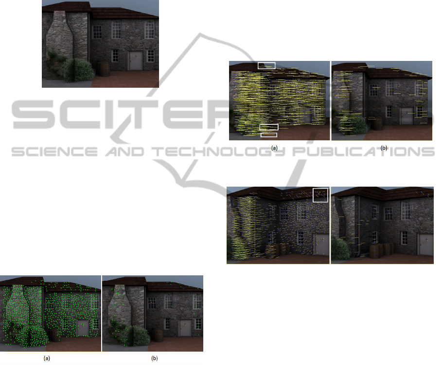
The video called Home (Figure 2) is a 640x480 pix-

els resolution video and it has 102 frames over ten

seconds.

Figure 2: Synthetic video - Home.

The initial step of the methodology consists in

tracking the scene. The best 1024 features were pro-

vided (Figure 3a) according with the GFTT classiﬁ-

cation. The next step is to decompose the input data

provided by the tracker in (X, Y) as shown in the sec-

tion 3.5. It is important to perceive that in Figure 4,

the paths the features made basically follow a hori-

zontal movement, therefore it could be applied the

SKen test only on the X axis; it would considerably

decrease the processing time. Finally, the last step is

to apply the SKen in the 1024 features initially pro-

vided by the tracker and to sort the obtained p-values

as it increases. The lower the p-value, the smoother is

the path.

Figure 3: (a) Frame 1: Synthetic video - Home (b) Frame

1(SKen): Synthetic video - Home

When applying the methodology, the scene is re-

constructed using only the ﬁrst 120 features, which

represents an 88.3 % drop concerning all features ini-

tially tracked. In other words, the scene was recon-

structed using the 120 smoother features and within

those 120 features there are thirty features that were

tracked between the ﬁrst and second keyframe. The

smoother features evidenced by the SKen test can be

seen in Figure 3b.

If visually compared, it can be noticed that

throughout the tracked video with 1024 features,

some features did not present a smooth movement, as

shown in Figure 4a. The white rectangles in the ﬁgure

emphasize the most relevant non-smooth paths.

When adopted only the 120 features given by the

SKen test, these non-smooth features disappeared, as

shown in Figure 4b. This is due to the fact that these

features had a less smooth behavior, i.e. in the test

they presented a p-value higher than the ﬁnal 120 se-

lected. Another example of non-smoothness also oc-

curs in Figure 5a. These same features do not appear

in the video sequence when using the SKen (Figure

5b), they also were classiﬁed as less smooth than the

selected by the SKen test.

Figure 4: (a) Frame 11: Synthetic video - Home (b) Frame

11 (SKen):Synthetic video - Home.

Figure 5: (a) Frame 88: Synthetic video - Home (b) Frame

88 (SKen): Synthetic video - Home.

As one the results of the methodology is the reduc-

tion of the number of features and thereby reducing

the processing time, the 3D mesh may be less detailed

than the one with the points initially tracked. How-

ever, as mentioned earlier in this section, the most im-

portant requirements are both the reprojection errors

frame by frame and a well-estimated camera pose.

Nevertheless, even with a restricted number of fea-

tures, the 3D mesh was not impaired. The mesh and

3D camera path can be seen in Figure 6.

Using the initial 1024 features, the video Home

presented an average reprojection error frame by

frame of 0.2327 pixels. When executed the SKen test,

the reconstructed scene had an average reprojection

error of 0.2180 pixels, which means it decreased by

6.3%. The reprojection errors frame by frame can be

seen in Figure 7.

Once the average reprojection error of all features

and the average error between features used by the

VISAPP2014-InternationalConferenceonComputerVisionTheoryandApplications

206

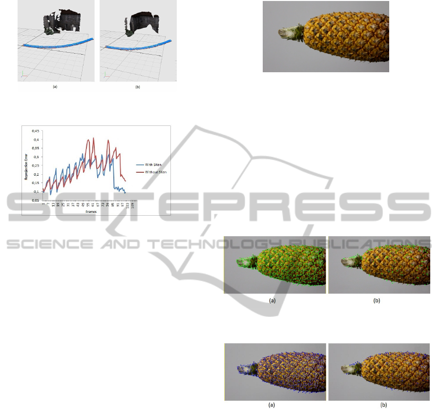
Figure 6: (a) 3D Reconstruction: Synthetic video - Home

(b) 3D Reconstruction (SKen): Synthetic video - Home.

Figure 7: Synthetic video - Home: Reprojection error frame

by frame.

SKen were very close to each other (only 6.3 % differ-

ence), it was performed the Wilcoxon test (Hollander

and Wolfe, 1999) for comparing these means. This

test was selected because the generated reprojection

error frame by frame, in this case, does not satisfy

aspects of normal distribution (Hollander and Wolfe,

1999). With the Wilcoxon test it was obtained a p-

value of 0.3764, which indicates that there is no sig-

niﬁcant difference between the mean errors, i.e. the

reconstructed scene, when using the SKen test, did

not affect the reprojection error.

It must be highlighted that the Home video is a

synthetic composition; therefore it presents a low-

noise sequence. The main gain in this scenario is due

to a signiﬁcant restriction in the amount of features

used, thereby also reducing the processing time of the

RANSAC. Even with an 88% decrease in the features,

it was statistically maintained the same reprojection

error.

The test was executed in an Intel(R) Core(TM) i3-

2120 CPU with 3.3GHz. The average execution time

of the SKen in C was approximately 0.4 milliseconds.

That is, the increment in runtime in C is practically

imperceptible.

4.2 Real Video

The second experiment used a real video called

Pineapple, which has been recorded with a 960x544

pixels resolution and composed of 164 frames over

ﬁve seconds (Figure 8).

As well as in previous case, the initial step of the

Figure 8: Real Video - Pineapple.

method consists in tracking the scene. The best 2000

features were provided (Figure 9a) according to the

GFTT classiﬁcation. The next step is to decompose

the input data given by the tracker (X, Y) as shown in

section 3.5.

It is important to notice that, in the Figure 10,

the paths the features made basically follow vertical

movement; therefore it could be applied the SKen test

only on the Y axis. Again, the last step is to apply

the SKen in the 2000 features initially provided by

the tracker and to sort the obtained p-values as it in-

creases.

Figure 9: (a)Frame 1: Real Video - Pineapple (b) Frame 1

(SKen): Real Video - Pineapple.

Figure 10: (a) Frame 12:Real Video - Pineapple (b) Frame

12 (SKen): Real Video - Pineapple.

According to the Algorithm 2, the scene might be

reconstructed using only the ﬁrst 153 features, which

represents a 92.3% decrease regarding the total fea-

tures that were initially tracked. In other words, the

scene was reconstructed using the smoother 153 fea-

tures and within those 153 features there are thirty

features that were tracked between the ﬁrst and sec-

ond keyframe. The smoother features evidenced by

the SKen test can be seen in Figure 9b.

The resulting 3D mesh with the points selected

by the SKen test has shown slightly different changes

even though it used only 7.6% of the initial features.

The mesh and the 3D camera path can be seen in Fig-

ure 11.

Using the initial 2000 features, the Pineapple

SKen:AStatisticalTestforRemovingOutliersinOpticalFlow-A3DReconstructionCase

207

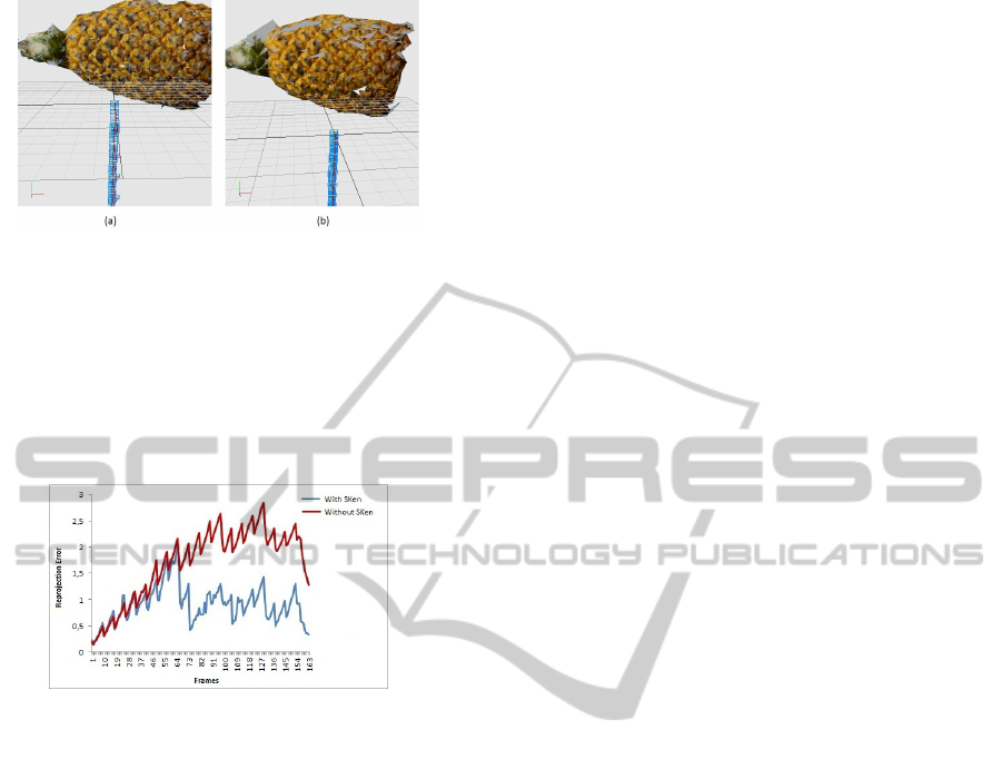
Figure 11: (a) 3D Reconstruction: Real Video - Pineapple

(b) 3D Reconstruction (SKen): Real Video - Pineapple.

video presented an average reprojection error frame

by frame of 1.689 pixels. When used the SKen test,

the reconstructed scene had an average reprojection

error of 0.90 pixels, which means a signiﬁcant 46.9%

drop. The reprojection errors frame by frame can be

seen in Figure 12.

Figure 12: Real Video - Pineapple: Reprojection error

frame by frame.

Although the difference between the reprojection

errors was considerably high, and shown in Figure 12

(mainly from the frame 70 onward), it was performed

the Wilcoxon test (Hollander and Wolfe, 1999) for

statistical conﬁrmation of this difference. As well as

in the previous case, this test was adopted because

the reprojection error frame by frame produced in

this case does not meet the conditions of the normal

distribution (Hollander and Wolfe, 1999). With the

Wilcoxon test it was obtained a p-value smaller than

−5

, which indicates that there is signiﬁcant differ-

ence between the mean errors, i.e. the reconstructed

scene reduced the average error of reprojection with

the SKen test.

The same experiment setup was deﬁned, as well

as the hardware speciﬁcations. When implemented in

C the average processing time was approximately 0.5

milliseconds. That is, the increment in execution time

in C is practically imperceptible.

Considering this last scenario, applying the SKen

caused a 92.3% drop in the number of features. It

practically did not change the pipeline total runtime

and decreased by 46.9% the reprojection error frame

by frame.

5 CONCLUSIONS

This work presented important results concerning a

3D reconstruction pipeline by adopting a new tech-

nique called SKen. Although this method may reduce

the amount of features during the tracking stage, it is

not its objective; this is a consequence. The focus of

the SKen is the selection of the best features. Thereat,

the pipeline calculations can be more accurate and

thus more reliable scene reconstructions scenes will

be produced.

The two case studies present evidence that fea-

tures that performed smooth paths are inlier features.

This correlation can be conﬁrmed by analyzing the

reprojection error behavior; with the SKen selected

features, reprojection errors either decreased or re-

mained the same. Furthermore, it is also shown that it

was not necessary to use the total amount of features

initially tracked, since the same reconstruction results

were achieved with less features and minor errors.

While in the synthetic and less noisy case the fea-

tures selected by the SKen test achieved the same av-

erage reprojection error than the features originally

tracked, this result was obtained by using only 11.7%

of features provided by the tracker. For the real case

with higher noise, the average reprojection error de-

creased by 46.9% and this result was obtained using

only 7.7% of features provided by the tracker.

The main challenge of this investigation was to de-

velop a methodology for obtaining results in real-time

as well as it should not compromise the performance

of the 3D reconstruction pipeline. The implementa-

tion of the SKen in C obtained an approximate av-

erage execution time of 0.5 milliseconds for a scene

with 2000 features. It represents only 1.5% of what

is necessary for meeting real-time requirements (ap-

proximately 33.3 milliseconds).

Finally, one of the most important features of the

proposed methodology is that the user does not need

to enter any parameters. Thus, this paper presented

an automatic and deterministic method in a way that

it does not need user intervention in order to remove

outliers.

REFERENCES

Barbosa, R. L. (2006). Caminhamento Fotogramtrico Uti-

lizando o Fluxo ptico Filtrado. PhD thesis, UNESP.

Bolfarine, H. and Bussab, W. O. (2005). Elementos de

Amostragem. Editora Edgard Blucher, So Paulo.

Bouguet, J. Y. (2000). Pyramidal implementation of the

lucas kanade feature tracker: Description of the algo-

rithm. Technical report, Intel Corporation.

VISAPP2014-InternationalConferenceonComputerVisionTheoryandApplications

208

Bussab, W. and Morettin, P. (2002). Estatstica Bsica. Edi-

tora Saraiva.

Choi, J. and Medioni, G. (2009). Starsac: Stable random

sample consensus for parameter estimation. IEEE In-

ternational Conference on Computer Vision and Pat-

tern Recognition, pages 675–682.

Farias, T. S. M. C. (2012). Metodologia para Reconstruo

3D Baseada em Imagens. PhD thesis, UFPE.

Fischler, M. A. and Bolles, R. C. (1987). Random sample

consensus: A paradigm for model ﬁtting with appli-

cations to image analysis and automated cartography.

Morgan Kaufmann Publishers Inc.

Furukawa, Y. and Ponce, J. (2010). Accurate, dense and ro-

bust multiview stereopsis. IEEE Transactions on Pat-

tern Analysis and Machine Intelligence, 32(8):1362–

1376.

Hartley, R. I. and Zisserman, A. (2004). Multiple View Ge-

ometry in Computer. 2nd ed. Cambridge University

Press, ISBN: 0521540518.

Hming, K. and Peters, G. (2010). The structure from motion

reconstruction pipeline: a survey with focus on short

image. Kybernetika.

Hollander, M. and Wolfe, D. A. (1999). Nonparametric

Statistical Methods, 2nd Edition. Wiley-Interscience,

2 edition.

James, B. R. (2002). Probabilidade: Um curso em nvel

intermedirio. IMPA, Rio de Janeiro.

Lucas, B. D. and Kanade, T. (1981). An iterative image

registration technique with an application to stereo

vision (ijcai). In Proceedings of the 7th Interna-

tional Joint Conference on Artiﬁcial Intelligence (IJ-

CAI ’81), pages 674–679.

Nist

er, D. (2003). Preemptive ransac for live structure and

motion estimation. In Proceedings of the Ninth IEEE

International Conference on Computer Vision - Vol-

ume 2, ICCV ’03, pages 199–, Washington, DC, USA.

IEEE Computer Society.

Pollefeys, M. (1999). Self-calibration and metric 3D recon-

struction uncalibrated image sequeces. PhD thesis,

ESAT-PSI.

Rodehorst, V. and Hellwich, O. (2006). Genetic algorithm

sample consensus (gasac) - a parallel strategy for ro-

bust parameter estimation. In Computer Vision and

Pattern Recognition Workshop, 2006. CVPRW ’06.

Conference on, page 103.

Rousseeuw, P. and Leroy, A. (1987). Robust Regression and

Outlier Detection. John Wiley.

Shi, J. and Tomasi, C. (1994). Good features to track. In

1994 IEEE Conference on Computer Vision and Pat-

tern Recognition (CVPR’94), pages 593 – 600.

Torr, P. H. S. and Zisserman, A. (2000). Mlesac: A new

robust estimator with application to estimating image

geometry. Computer Vision and Image Understand-

ing, 78:2000.

SKen:AStatisticalTestforRemovingOutliersinOpticalFlow-A3DReconstructionCase

209