
mC-ReliefF
An Extension of ReliefF for Cost-based Feature Selection
Ver´onica Bol´on-Canedo, Beatriz Remeseiro, Noelia S´anchez-Maro˜no and Amparo Alonso-Betanzos
Department of Computer Science, University of A Coru˜na, Campus de Elvi˜na s/n, A Coru˜na 15071, Spain
Keywords:
Cost-based Feature Selection, Machine Learning, Filter Methods, Support Vector Machine.
Abstract:
The proliferation of high-dimensional data in the last few years has brought a necessity to use dimensionality
reduction techniques, in which feature selection is arguably the favorite one. Feature selection consists of
detecting relevant features and discarding the irrelevant ones. However, there are some situations where the
users are not only interested in the relevance of the selected features but also in the costs that they imply, e.g.
economical or computational costs. In this paper an extension of the well-known ReliefF method for feature
selection is proposed, which consists of adding a new term to the function which updates the weights of the
features so as to be able to reach a trade-off between the relevance of a feature and its associated cost. The
behavior of the proposed method is tested on twelve heterogeneous classification datasets as well as a real
application, using a support vector machine (SVM) as a classifier. The results of the experimental study show
that the approach is sound, since it allows the user to reduce the cost significantly without compromising the
classification error.
1 INTRODUCTION
Feature selection in data mining has been an active
research area for decades. This technique is applied
to reduce the dimensionality of the original data and
improve learning performance. In a situation of hav-
ing a large number of features, many of them may be
irrelevant or redundant. Feature selection carries out
the process of discarding irrelevant or redundant fea-
tures. By removing these unnecessary features in the
data and thus generating a smaller set of features with
more discriminant power, feature selection brings the
immediate effects of speeding up data mining algo-
rithms, improving performance, and enhancing model
comprehensibility (Zhao and Liu, 2012).
Feature selection methods can be divided into
wrappers, filters and embedded methods (Guyon
et al., 2006). The filter model relies on the general
characteristics of training data and carries out the fea-
ture selection process as a pre-processing step with
independence of the induction algorithm. The embed-
ded methods generally perform feature selection in
the process of training and are specific to given learn-
ing machines. Wrappers, in turn, involve optimizing
a predictor as part of the selection process. Wrappers
and embedded methods tend to obtain better perfor-
mances but at the expense of being very time consum-
ing and having the risk of overfitting when the sample
size is small. In contrast, filters are faster, easier to
implement, scale up better than wrappers and embed-
ded methods, and can be used as a pre-processing step
before applying other more complex methods.
The most common approaches followed by fea-
ture selection methods are to find either a subset of
features that maximizes a given metric or either an
ordered ranking of the features based on this metric.
However,there are some situations where a user is not
only interested in maximizing the merit of a subset of
features, but also in reducing costs that may be associ-
ated to features. For example, for medical diagnosis,
symptoms observed with the naked eye are costless,
but each diagnostic value extracted by a clinical test
comes with its own cost and risk. Another example
is the computational time required to deal with one or
another feature, especially in real-time applications.
Surprisingly, this topic has not been the focus of much
attention for feature selection researchers.
This paper presents an attempt to fill this gap
by proposing a filter-based feature selection method,
called mC-ReliefF, to deal with cost-based feature
selection. This method can be used to achieve a
trade-off between the filter metric and the cost as-
sociated to the selected features, in order to select
relevant features with a low associated cost. mC-
42
Bolón-Canedo V., Remeseiro B., Sánchez-Maroño N. and Alonso-Betanzos A..
mC-ReliefF - An Extension of ReliefF for Cost-based Feature Selection.
DOI: 10.5220/0004756800420051
In Proceedings of the 6th International Conference on Agents and Artificial Intelligence (ICAART-2014), pages 42-51
ISBN: 978-989-758-015-4
Copyright
c
2014 SCITEPRESS (Science and Technology Publications, Lda.)

ReliefF is based on the well-known ReliefF method
(Kononenko, 1994), which can be applied to both
continuous and discrete problems, includes interac-
tion among features, and may capture local depen-
dencies that other methods miss. To evaluate the per-
formance of the proposed method, twelve datasets
were employed, as well as a real application, show-
ing promising results.
2 THE RATIONALE OF THE
APPROACH
New feature selection methods are continuously
emerging, being successfully applied to different ar-
eas (Inza et al., 2004; Forman, 2003; Lee et al., 2000).
However, the great majority of them only focus on re-
moving unnecessary features from the point of view
of maintaining the performance, but do not take into
account the possible different costs for obtaining the
features. So, our aim will be to maintain performance,
but also trying to balance the costs of the selected fea-
tures.
The cost associated with a feature may come from
different origins. For example, the cost can be related
to computational issues. In the medical imaging field,
extracting a feature from a medical image can have a
high computational cost. In other cases, such as real-
time applications, the space complexity is negligible,
but the time complexity is very important (Feddema
et al., 1991).
A second typical scenario where features have an
associated cost is medical diagnosis. A pattern in
this case consists of observable symptoms (which are
costless, such as age, sex, etc.) along with the re-
sults of some diagnostic tests (usually with associ-
ated costs and risks). For example, an invasive ex-
ploratory surgery is much more expensive and risky
than a blood test (Yang and Honavar, 1998).
Although features with a related cost can be found
in many real-life applications, this has not been the
focus of much attention for machine learning re-
searchers. To the best knowledge of the authors, there
are only a few attempts in the literature to deal with
this issue (Feddema et al., 1991; Huang and Wang,
2006; Sivagaminathan and Ramakrishnan, 2007; Min
et al., 2013). Most of these methods, though, have
the disadvantage of being computationally expensive
by having interaction with the classifier, which pre-
vents their use in large datasets, a trending topic in
the past few years (Han et al., 2006). A quick exami-
nation of the most popular machine learning and data
mining tools revealed that no cost aware methods can
be found. In fact, in Weka (Hall et al., 2009) we can
only find some methods that address the problem of
cost associated to the instances (not to the features).
RapidMiner (Mierswa et al., 2006) does include some
methods to handle cost related to features, but they are
quite simple. One of them selects the attributes which
have a cost value which satisfies a given condition and
another one just selects the k attributes with the lowest
cost.
In this paper the idea is to modify the well-known
filter ReliefF, which (1) can be applied in many dif-
ferent situations, (2) has low bias, (3) includes inter-
action among features and (4) has linear dependency
on the number of features. Therefore, the proposed
mC-ReliefF will be suitable even for application to
datasets with a great number of input features such as
microarray DNA data.
3 PROPOSED METHOD
Relief(Kira and Rendell, 1992) and its multiclass ex-
tension, ReliefF(Kononenko, 1994), are supervised
feature weighting algorithms included in the filter ap-
proach. The key point is to estimate the quality of
attributes according to how well their values distin-
guish between instances that are near to each other
(Robnik-
ˇ
Sikonja and Kononenko, 2003). Therefore,
given a randomly selected instance R
i
, the Relief al-
gorithm searches for its two nearest neighbors: one
for the same class, nearest hit H, and the other from
the different class, nearest miss M. In the next subsec-
tions ReliefF will be presented in detail as well as the
modification introduced in this research.
3.1 ReliefF
The ReliefF algorithm is not limited to two class
problems, is more robust, and can deal with incom-
plete and noisy data. As the original ReliefF algo-
rithm, ReliefF randomly selects an instance R
i
, but
then searches for k of its nearest neighbors from the
same class, nearest hits H
j
, and also k nearest neigh-
bors from each one of the different classes, nearest
misses M
j
(C). It updates the quality estimation W[A]
for all attributes A depending on their values for R
i
,
hits H
j
and misses M
j
(C). If instances R
i
and H
j
have
different values of the attribute A, then this attribute
separates instances of the same class, which clearly
is not desirable, and thus the quality estimation W[A]
has to be decreased. On the contrary, if instances R
i
and M
j
have different values of the attribute A for a
class then the attribute A separates two instances with
different class values which is desirable so the quality
estimation W[A] is increased. Since ReliefF considers
mC-ReliefF-AnExtensionofReliefFforCost-basedFeatureSelection
43

multiclass problems, the contribution of all the hits
and all the misses is averaged. Besides, the contribu-
tion for each class of the misses is weighted with the
prior probability of that class P(C) (estimated from
the training set). The whole process is repeated m
times (where m is a user-defined parameter) and can
be seen in Algorithm 1.
Algorithm 1: Pseudo-code of ReliefF algorithm.
Data: training set D, iterations m, attributes a
Result: the vector W of estimations of the
qualities of attributes
1 set all weights W[A] := 0
2 for i ← 1 to m do
3 randomly select an instance R
i
4 find k nearest hits H
j
5 for each class C 6= class(R
i
) do
6 from class C find k nearest misses
M
j
(C)
end
end
7 for f ← 1 to a do
8 W[ f] := W[ f] −
∑
k
j=1
dif f( f,R
i
,H
j
)
(m·k)
+
∑
C6=class(R
i
)
h
P(C)
1−P(class(R
i
))
∑
k
j=1
dif f( f,R
i
,M
j
(C))
i
(m·k)
end
The function dif f(A, I
1
, I
2
) calculates the differ-
ence between the values of the attribute A for two in-
stances, I
1
and I
2
. If the attributes are nominal, it is
defined as:
dif f(A, I
1
, I
2
) =
(
0; value(A, I
1
) = value(A, I
2
)
1; otherwise
3.2 mC-ReliefF
The modification of ReliefF we propose in this re-
search, called minimum Cost ReliefF (mC-ReliefF),
consists of adding a term to the quality estimation
W[ f] to take into account the cost of the features, as
can be seen in (1).
W[ f] := W[ f] −
∑
k
j=1
dif f( f,R
i
,H
j
)
(m·k)
+
∑
C6=class(R
i
)
h
P(C)
1−P(class(R
i
))
∑
k
j=1
dif f( f,R
i
,M
j
(C))
i
(m·k)
−
λ·Z
f
(m·k)
,
(1)
where Z
f
is the cost of the feature f, and λ is a free
parameter introduced to weight the influence of the
cost in the quality estimation of the attributes.
The parameter λ is a positive real number. If λ is
0, the cost is ignored and the method works as the reg-
ular ReliefF. If λ is between 0 and 1, the influence of
the cost is smaller than the relevance of the feature. If
λ = 1 both relevance and cost have the same influence
and if λ > 1, the influence of the cost is greater than
the influence of the relevance. This parameter needs
to be left as a free parameter because determining the
importance of the cost is highly dependent of the do-
main. For example, in a medical diagnosis, the accu-
racy cannot been sacrificed in favor of reducing eco-
nomical costs. On the contrary, in some real-time ap-
plications, a slight decrease in classification accuracy
is allowed in order to reduce the processing time sig-
nificantly. An example of this behavior will be shown
on a real scenario in Section 6.
4 EXPERIMENTAL STUDY
The experimental study is performed over twelve dif-
ferent datasets, as can be seen in Table 1, all of them
available for download
1
. To test the performance of
the proposed method, we first selected four classi-
cal dataset from the UCI repository (Asuncion and
Newman, 2007) with a larger number of samples than
of features (Table 1, rows 1-4), and four microarray
datasets, which are characterized for having a much
larger number of features than samples (Table 1, rows
5-8). Since these datasets do not have intrinsic cost
associated, random cost for their input attributes has
been generated. For each feature, the cost was gen-
erated as a random number between 0 and 1. For in-
stance, Table 2 displays the random costs generated
for each feature of Magic04 dataset.
The main feature of the last four datasets is that
they have intrinsic cost associated to the input at-
tributes, so that will be an opportunity for checking if
the proposed method works correctly when the costs
are not randomly generated. For the sake of fairness,
these costs have been normalized between 0 and 1. To
the best knowledge of the authors, no more datasets
with cost exist publicly available.
Overall, the chosen classification datasets are very
heterogeneous. They present a diverse number of
classes, ranging from 2 to 26. The number of sam-
ples and features ranges from single digits to the or-
der of thousands. Notice that microarray datasets
have a much larger number of features than samples,
which poses a big challenge for feature selection re-
searchers, whilst the remaining datasets have a larger
1
The microarray datasets are available on http://www.-
broadinstitute.org/cgi-bin/cancer/datasets.cgi; the remain-
ing datasets on http://archive.ics.uci.edu/ml/datasets.html
ICAART2014-InternationalConferenceonAgentsandArtificialIntelligence
44

Table 1: Description of the datasets.
Dataset No. features No. samples No. classes
Letter 16 20000 26
Magic04 10 19020 2
Sat 36 4435 6
Waveform 21 5000 3
CNS 7129 60 2
Colon 2000 62 2
DLBCL 4026 47 2
Leukemia 7129 72 2
Hepatitis 19 155 2
Liver 6 345 2
Pima 8 768 2
Thyroid 20 3772 3
Table 2: Random costs of the features of Magic04 dataset.
Feature Cost
1 0.3555
2 0.2519
3 0.0175
4 0.9678
5 0.6751
6 0.4465
7 0.8329
8 0.1711
9 0.6077
10 0.7329
number of samples than features. This variety of
datasets allows for a better understanding of the be-
havior of the proposed mC-ReliefF.
The experiments consist of applying the proposed
mC-ReliefF over those datasets. The aim of the ex-
periment is to study the behavior of the method under
the influence of the λ parameter. The performance is
evaluated in terms of both the total cost of the selected
features and the classification error obtained by a sup-
port vector machine (Burges, 1998) (SVM) classifier
estimated under a 10-fold cross-validation. This tech-
nique consists of dividing the dataset into 10 subsets
and repeating the process 10 times. Each time, 1 sub-
set is used as the test set and the other 9 subsets are
put together to form the training set. Finally, the av-
erage error and cost across all 10 trials are computed.
It is expected that the larger the λ, the lower the cost
and the higher the error, since increasing λ gives more
weight to cost at the expense of reducing the impor-
tance of the relevance of the features. Moreover, a
Kruskal-Wallis statistical test and a multiple compari-
son test (based on Tukey’s honestly significant differ-
ence criterion) (Hochberg and Tamhane, 1987) have
been run on the errors and cost obtained. These re-
sults could help the user to choose the value of the λ
parameter.
5 EXPERIMENTAL RESULTS
This section presents the average cost and error for
several values of λ. Since mC-ReliefF returns an or-
dered ranking of features, a threshold is required. For
the datasets with a notable larger number of samples
than features (Table 1, rows 1-4, 9-12), experiments
were executed retaining 25%, 50% and 75% of the
original features. For the microarray datasets (Table
1, rows 5-8), which have a much larger number of
features than samples, we retain 0.50%, 1% and 2%
of the original input features.
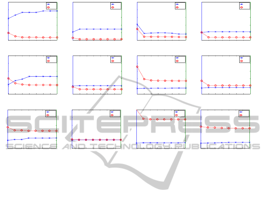
Figure 1 reports the results for the classical
datasets (rows 1-4 in Table 1) where the cost was ran-
domly added. Several values of λ were tested, up to
λ = 10, but in the figures we are only showing val-
ues until λ = 2, since cost and error remained con-
stant for the remaining values. The behavior expected
when applying mC-ReliefF is that the higher the λ,
the lower the cost and the higher the error. As for
the number of features retained, it is expected that the
higher the percentage of features used, the lower the
error and the higher the cost. In general, when in-
creasing the value of λ, the error either is higher or
constant, whilst the cost decreases until a certain level
of λ and from there on it does not vary. There is a
exception for this behavior with Sat dataset retaining
25% of features (see Figure 1(c)). In this case, not
only is the cost decreasing, but also the error, which
is better than expected. At this point, it is necessary to
remind that mC-ReliefF is a filter approach, with the
benefits of being fast and computationally inexpen-
sive because of the classifier-independence. However,
this independencemay cause that the selected features
would not be the more suitable for a given classifier
to obtain the highest accuracy. In some cases, forcing
a filter to select features according to another crite-
rion (such as reducing the cost), can bring unexpected
classification results.
The Kruskal-Wallis tests run on the results re-
vealed diverse situations. For Letter dataset (with
50% and 75% of features, Figures 1(e) and 1(i)) and
Magic04 with 25% of features (Figure 1(b)), it is
not possible to select a value of λ such that the cost
decreases significantly at the same time that the er-
ror does not worsen significantly. For these cases,
the user has to decide between reducing the cost (at
the expense of a slightly decrease in performance)
or maintaining the performance (at the expense of a
higher cost). Nevertheless, for the remaining combi-
nations of dataset and percentage of features, there is
always a value of λ such that the cost is significantly
reduced whilst the error does not significantly change
(compared with λ = 0 which is the regular ReliefF).
mC-ReliefF-AnExtensionofReliefFforCost-basedFeatureSelection
45
0 0.15 0.25 0.40 0.5 0.75 1 2
0
0.2
0.4
0.6
0.8
1
λ
Error
0
3
6
9
12
15
Cost
Error
Cost
(a) Letter 25%
0 0.15 0.25 0.40 0.5 0.75 1 2
0
0.2
0.4
0.6
0.8
1
λ
Error
0
3
6
9
12
15
Cost
Error
Cost
(b) Magic04 25%
0 0.15 0.25 0.40 0.5 0.75 1 2
0
0.2
0.4
0.6
0.8
1
λ
Error
0
3
6
9
12
15
Cost
Error
Cost
(c) Sat 25%
0 0.15 0.25 0.40 0.5 0.75 1 2
0
0.2
0.4
0.6
0.8
1
λ
Error
0
3
6
9
12
15
Cost
Error
Cost
(d) Waveform 25%
0 0.15 0.25 0.40 0.5 0.75 1 2
0
0.2
0.4
0.6
0.8
1
λ
Error
0
3
6
9
12
15
Cost
Error
Cost
(e) Letter 50%
0 0.15 0.25 0.40 0.5 0.75 1 2
0
0.2
0.4
0.6
0.8
1
λ
Error
0
3
6
9
12
15
Cost
Error
Cost
(f) Magic04 50%
0 0.15 0.25 0.40 0.5 0.75 1 2
0
0.2
0.4
0.6
0.8
1
λ
Error
0
3
6
9
12
15
Cost
Error
Cost
(g) Sat 50%
0 0.15 0.25 0.40 0.5 0.75 1 2
0
0.2
0.4
0.6
0.8
1
λ
Error
0
3
6
9
12
15
Cost
Error
Cost
(h) Waveform 50%
0 0.15 0.25 0.40 0.5 0.75 1 2
0
0.2
0.4
0.6
0.8
1
λ
Error
0
3
6
9
12
15
Cost
Error
Cost
(i) Letter 75%
0 0.15 0.25 0.40 0.5 0.75 1 2
0
0.2
0.4
0.6
0.8
1
λ
Error
0
3
6
9
12
15
Cost
Error
Cost
(j) Magic04 75%
0 0.15 0.25 0.40 0.5 0.75 1 2
0
0.2
0.4
0.6
0.8
1
λ
Error
0
3
6
9
12
15
Cost
Error
Cost
(k) Sat 75%
0 0.15 0.25 0.40 0.5 0.75 1 2
0
0.2
0.4
0.6
0.8
1
λ
Error
0
3
6
9
12
15
Cost
Error
Cost
(l) Waveform 75%
Figure 1: Error / cost plots of first block of datasets for different values of λ, and different percentages of features (25%, 50%
and 75%).
For the sake of brevity, not all the cases can be ana-
lyzed in detail, but it is worth commenting on some
specific cases. For Letter dataset with 25% of fea-
tures (Figure 1(a)), λ = 0.25 allows the user to reduce
significantly the cost without compromising the clas-
sification performance, and the same happens with
Magic04 (50% and 75% of features) and Waveform
(25% and 50% of features). For datasets Sat (50%
and 75% of features) and Waveform with 75% of fea-
tures, λ = 0.40 obtains also a reduction in cost whilst
maintaining the classification error with no significant
changes. The case of Sat with 25% of features (Figure
1(c)) is of special interest, since λ = 0.75 produces a
significant reduction in cost and error at the same time
(compared with regular ReliefF).
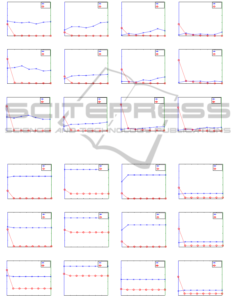
After checking the adequacy of the proposed
method on classical datasets, mC-ReliefF is tested
against DNA microarray datasets (Table 1, rows 9-
12), with much more features than samples. As ex-
pected, cost decreases as λ increases, and since these
datasets have a much larger number of input attributes
than the previous ones, the cost values experiment
larger variabilities (see Figure 2). For this reason, val-
ues of λ up to 10 are shown in these graphics. For all
the microarray datasets and percentages of features,
the Kruskal-Wallis test revealed that λ = 1 reduces
significantly the cost (compared to regular ReliefF)
with no meaningful changes in classification error.
So far, we have demonstrated the adequacy of mC-
ReliefF on datasets where the cost was added ran-
domly to the attributes. Figure 3 shows the average
cost and error for the last four datasets in Table 1,
the ones which came with associated cost. As for the
classical datasets, the figures are only showing val-
ues until λ = 2, since cost and error remained con-
stant for the remaining values. The behavior expected
when applying mC-ReliefF is that the higher the λ,
the lower the cost and the higher the error. As for
the number of features retained, it is expected that the
higher the percentage of features used, the lower the
error and the higher the cost. The results displayed in
Figure 3, in fact show that cost value behaves as ex-
pected (although the magnitude of the cost does not
change too much because these datasets have a very
small number of features). The error, however, re-
mains constant in most of the cases. The Kruskal-
Wallis statistical test run on the results demonstrates
that the errors are not significantly different for any
value of λ for all the different combinations of dataset
and percentage of features. For the cost, however,
there are statistical differences between λ = 0 (in this
case the cost has no influence, so it is the regular Re-
liefF) and the remaining values of λ, except for Pima
dataset with 75% of features (Figure 3(k)), with no
ICAART2014-InternationalConferenceonAgentsandArtificialIntelligence
46
0 0.5 0.75 1 2 5 10
0
0.2
0.4
0.6
0.8
1
λ
Error
0
10
20
30
40
50
Cost
Error
Cost
(a) CNS 0.50%
0 0.5 0.75 1 2 5 10
0
0.2
0.4
0.6
0.8
1
λ
Error
0
10
20
30
40
50
Cost
Error
Cost
(b) Colon 0.50%
0 0.5 0.75 1 2 5 10
0
0.2
0.4
0.6
0.8
1
λ
Error
0
10
20
30
40
50
Cost
Error
Cost
(c) DLBCL 0.50%
0 0.5 0.75 1 2 5 10
0
0.2
0.4
0.6
0.8
1
λ
Error
0
10
20
30
40
50
Cost
Error
Cost
(d) Leukemia 0.50%
0 0.5 0.75 1 2 5 10
0
0.2
0.4
0.6
0.8
1
λ
Error
0
10
20
30
40
50
Cost
Error
Cost
(e) CNS 1%
0 0.5 0.75 1 2 5 10
0
0.2
0.4
0.6
0.8
1
λ
Error
0
10
20
30
40
50
Cost
Error
Cost
(f) Colon 1%
0 0.5 0.75 1 2 5 10
0
0.2
0.4
0.6
0.8
1
λ
Error
0
10
20
30
40
50
Cost
Error
Cost
(g) DLBCL 1%
0 0.5 0.75 1 2 5 10
0
0.2
0.4
0.6
0.8
1
λ
Error
0
10
20
30
40
50
Cost
Error
Cost
(h) Leukemia 1%
0 0.5 0.75 1 2 5 10
0
0.5
1
λ
Error
0
50
100
Cost
Error
Cost
(i) CNS 2%
0 0.5 0.75 1 2 5 10
0
0.2
0.4
0.6
0.8
1
λ
Error
0
10
20
30
40
50
Cost
Error
Cost
(j) Colon 2%
0 0.5 0.75 1 2 5 10
0
0.2
0.4
0.6
0.8
1
λ
Error
0
10
20
30
40
50
Cost
Error
Cost
(k) DLBCL 2%
0 0.5 0.75 1 2 5 10
0
0.5
1
λ
Error
0
50
100
Cost
Error
Cost
(l) Leukemia 2%
Figure 2: Error / cost plots of second block of datasets (microarray datasets) for different values of λ, and different percentages
of features (0.50%, 1% and 2%).
0 0.15 0.25 0.40 0.5 0.75 1 2
0
0.1
0.2
0.3
0.4
0.5
λ
Error
0
1
2
3
4
5
Cost
Error
Cost
(a) Hepatitis 25%
0 0.15 0.25 0.40 0.5 0.75 1 2
0
0.1
0.2
0.3
0.4
0.5
λ
Error
0
1
2
3
4
5
Cost
Error
Cost
(b) Liver 25%
0 0.15 0.25 0.40 0.5 0.75 1 2
0
0.1
0.2
0.3
0.4
0.5
λ
Error
0
1
2
3
4
5
Cost
Error
Cost
(c) Pima 25%
0 0.15 0.25 0.40 0.5 0.75 1 2
0
0.1
0.2
0.3
0.4
0.5
λ
Error
0
1
2
3
4
5
Cost
Error
Cost
(d) Thyroid 25%
0 0.15 0.25 0.40 0.5 0.75 1 2
0
0.1
0.2
0.3
0.4
0.5
λ
Error
0
1
2
3
4
5
Cost
Error
Cost
(e) Hepatitis 50%
0 0.15 0.25 0.40 0.5 0.75 1 2
0
0.1
0.2
0.3
0.4
0.5
λ
Error
0
1
2
3
4
5
Cost
Error
Cost
(f) Liver 50%
0 0.15 0.25 0.40 0.5 0.75 1 2
0
0.1
0.2
0.3
0.4
0.5
λ
Error
0
1
2
3
4
5
Cost
Error
Cost
(g) Pima 50%
0 0.15 0.25 0.40 0.5 0.75 1 2
0
0.1
0.2
0.3
0.4
0.5
λ
Error
0
1
2
3
4
5
Cost
Error
Cost
(h) Thyroid 50%
0 0.15 0.25 0.40 0.5 0.75 1 2
0
0.1
0.2
0.3
0.4
0.5
λ
Error
0
1
2
3
4
5
Cost
Error
Cost
(i) Hepatitis 75%
0 0.15 0.25 0.40 0.5 0.75 1 2
0
0.1
0.2
0.3
0.4
0.5
λ
Error
0
1
2
3
4
5
Cost
Error
Cost
(j) Liver 75%
0 0.15 0.25 0.40 0.5 0.75 1 2
0
0.1
0.2
0.3
0.4
0.5
λ
Error
0
1
2
3
4
5
Cost
Error
Cost
(k) Pima 75%
0 0.15 0.25 0.40 0.5 0.75 1 2
0
0.1
0.2
0.3
0.4
0.5
λ
Error
0
1
2
3
4
5
Cost
Error
Cost
(l) Thyroid 75%
Figure 3: Error / cost plots of third block of datasets (datasets with associated cost) for different values of λ, and different
percentages of features (25%, 50% and 75%).
mC-ReliefF-AnExtensionofReliefFforCost-basedFeatureSelection
47

significant differences among the values of λ. This
fact is very interesting, since it means that for these
datasets, we are able to reduce the cost significantly
without increasing the error, which was the goal of
this research.
To sum up, the proposed mC-ReliefF has been
tested on 12 different datasets, covering a wide range
of data conditions. For each dataset, 3 different per-
centages of features were considered, which leads to a
total of 36 combinations. Only in 3 out of the 36 cases
tested, the user has to decide between favoring the re-
duction of cost or the error. In the remaining cases,
it is possible to reduce the cost associated to features
without compromising the classification error, which
is a very important improvement of the well-known
and widely-used ReliefF filter. Finally, the proposed
method will be applied to a real dataset in order to
check if the conclusions drawn in this section can be
extrapolated to real-life problems.
6 CASE OF STUDY: A REAL LIFE
PROBLEM
In this section we present a real-life problem where
the cost, in the form of computational time, needs to
be reduced. Evaporative dry eye (EDE) is a symp-
tomatic disease which affects a wide range of pop-
ulation and has a negative impact on their daily ac-
tivities, such as driving or working with computers.
Its diagnosis can be achieved by several clinical tests,
one of which is the analysis of the interference pat-
tern and its classification into one of the four cate-
gories defined by Guillon (Guillon, 1998) for this pur-
pose. A methodology for automatic tear film lipid
layer (TFLL) classification into one of these cate-
gories has been developed (Remeseiro et al., 2011),
based on color texture analysis. The co-occurrence
features technique (Haralick et al., 1973), as a texture
extraction method, and the Lab color space (McLaren,
1976) provide the highest discriminative power from
a wide range of methods analyzed. However, the
best accuracy results are obtained at the expense of a
too long processing time (38 seconds) because many
features have to be computed. This fact makes this
methodology unfeasible for practical applications and
prevents its clinical use. Reducing processing time is
a critical issue in this application which should work
in real-time in order to be used in the clinical routine.
Therefore, the proposed mC-ReliefF is applied in an
attempt to decrease the numberof features and, conse-
quently, the computational time without compromis-
ing the classification performance.
So, the adequacy of mC-ReliefF is now tested
on the real problem of TFLL classification using the
dataset VOPTICAL
I1 (VOPTICAL I1, 2012). This
dataset consists of 105 images (samples) belonging
to the four Guillon’s categories (classes). All these
images have been annotated by optometrists from the
Faculty of Optics and Optometry of the University
of Santiago de Compostela (Spain). The methodol-
ogy for TFLL classification proposed in (Remeseiro
et al., 2011) consists of extracting the region of inter-
est (ROI) of an input image, and analyzing it based
on color and texture information. Thus, the ROI in
the RGB color space is transformed to the Lab color
space and the texture of its three components of color
(L, a and b) is analyzed. For texture analysis, the co-
occurrence features method generates a set of grey
level co-occurrence matrices (GLCM) for an spe-
cific distance and extracts 14 statistical measures from
their elements. Then, the mean and the range of these
14 statistical measures are calculated across matrices
and so a set of 28 features is obtained. Distances from
1 to 7 in the co-occurrence features method and the 3
components of the Lab color space are considered, so
the size of the final descriptor obtained from an input
image is: 28 features × 7 distances × 3 components =
588 features. Notice that the cost for obtaining these
features is not homogeneous. Features are vectorized
in groups of 28 related to distances and components
in the color space, where the higher the distance, the
higher the cost. Plus, each group of 28 features cor-
responds with the mean and range of the 14 statistical
measures calculated across the GLCMs. Among these
statistical measures, it was shown that computing the
so-called 14
th
statistic takes around 75% of the total
time. Therefore, we have to deal with a dataset with
a very variable cost (in this case, computational time)
associated to the input features.
Figure 4 (left) shows the average error and cost
after performing a 10-fold cross-validation for VOP-
TICAL
I1 dataset for different values of λ, for three
different sets of features. As expected, when λ in-
creases, the cost decreases and the error either raises
or is maintained. Regarding the different subsets of
features, the larger the number of features, the higher
the cost. The Kruskal-Wallis statistical test run on
the results demonstrated that there are no significant
differences among the errors achieved using different
values of λ, whilst using a λ ≥ 10 decreases signifi-
cantly the cost. This situation happens when retaining
25, 35 and 50 features.
Trying to shed light on the issue of which value of
λ is better for the problem at hand, the Pareto front
(Teich, 2001) for each alternative is showed in Figure
4 (right). In multi-objective optimization, the Pareto
front is defined as the border between the region of
ICAART2014-InternationalConferenceonAgentsandArtificialIntelligence
48
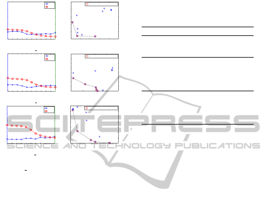
0 0.5 0.75 1 2 5 10 15 20 25 30
0
0.2
0.4
0.6
0.8
1
λ
Error
0
0.2
0.4
0.6
0.8
1
Cost
Error
Cost
(a) VOPTICAL I1 25 feats
0.12 0.14 0.16 0.18 0.2 0.22
0.05
0.1
0.15
0.2
0.25
0.3
Error
Cost
← λ=5
← λ=25
← λ=30
Points in the Pareto Front
(b) Pareto front 25 feats
0 0.5 0.75 1 2 5 10 15 20 25 30
0
0.2
0.4
0.6
0.8
1
λ
Error
0
0.2
0.4
0.6
0.8
1
Cost
Error
Cost
(c) VOPTICAL I1 35 feats
0.1 0.12 0.14 0.16 0.18
0.1
0.15
0.2
0.25
0.3
0.35
0.4
0.45
0.5
Error
Cost
← λ=5
← λ=10
← λ=15
← λ=20
← λ=30
Points in the Pareto Front
(d) Pareto front 35 feats
0 0.5 0.75 1 2 5 10 15 20 25 30
0
0.2
0.4
0.6
0.8
1
λ
Error
0
0.2
0.4
0.6
0.8
1
Cost
Error
Cost
(e) VOPTICAL I1 50 feats
0.1 0.12 0.14 0.16 0.18 0.2
0.2
0.25
0.3
0.35
0.4
0.45
0.5
Error
Cost
← λ=1
← λ=10
← λ=20
← λ=25
← λ=30
Points in the Pareto Front
(f) Pareto front 50 feats
Figure 4: Error / cost plots (left) and Pareto front (right) of
VOPTICAL
I1 dataset for different values of λ, and differ-
ent number of selected features (25, 35 and 50).
feasible points, for which all constraints are satisfied,
and the region of infeasible points. In this case, so-
lutions are constrained to minimize classification er-
ror and cost. In Figure 4 (right), points (values of λ)
in the Pareto front are marked with a red circle. All
those points are equally satisfying the constraints, and
it is decision of the user if he/she prefers to minimize
either the cost or the classification error. On the other
hand, choosing a value of λ outside the Pareto front
would imply to chose a worse solution than any in the
Pareto front.
Table 3 reports the classification error and cost (in
the form of time) for all the Pareto front points. No-
tice that as a 10-fold cross-validation was performed,
the final subset of selected features is the union of
the features selected in each fold, and that is why the
number of features in column 5 differs from the one
in the first column. As expected, the higher the λ, the
higher the error and the lower the time. The best re-
sult in terms of classification error was obtained with
λ = 5 when retaining 35 features per fold. In turn,
the lowest time was obtained with λ = 25 when re-
taining 25 features per fold, but at the expense of in-
creasing the error in almost 3%. In this situation, the
authors think that it is better to choose the best error
(λ = 5 retaining 35 features), since the difference in
time is not that important and in both cases is under
Table 3: Mean classification error(%), time (milliseconds),
and number of features in the union of the 10 folds for the
Pareto front points. Best error and time are marked in bold
face.
Feats λ Error Time Feats union
25
5 12.27 562.43 44
25 13.27 245.42 33
30 17.09 249.30 34
35
5 10.36 736.70 56
10 12.36 576.49 53
15 14.18 461.78 51
20 14.27 438.74 52
30 14.45 342.77 46
50
0 11.45 1398.28 83
10 11.45 806.26 74
20 14.27 559.00 66
25 15.18 510.47 64
30 18.18 488.11 62
1 second. The time required by previous approaches
which deal with TFLL classification prevented their
clinical use because they could not work in real time,
since extracting the whole set of features took 38 sec-
onds. Thus, since this is a real-time scenario where
reducing the computing time is a crucial issue, having
a processing time under 1 second leads to a signifi-
cant improvement. In this manner, the methodology
for TFLL classification could be used in the clinical
routine as a support tool to diagnose EDE.
7 CONCLUSIONS
In this paper a modification of the ReliefF filter for
cost-based feature selection, called mC-ReliefF, is
proposed. ReliefF is a well-known and widely used
filter, which has proven to be effective in diverse sce-
narios, such as both continuous and discrete prob-
lems, and includes interaction among features. The
extension proposed herein consists of allowing Reli-
efF to solve problems where it is interesting not only
to minimize the classification error, but also to reduce
costs that may be associated to input features. For this
purpose, a new term is added to the function which
updates the weights of the features so as to be able to
reach a trade-off between the relevance of a feature
and the cost that it implies. A new parameter, λ, is
introduced in order to adjust the influence of the cost
with respect to the influence of the relevance, allow-
ing users a fine tuning of the selection process balanc-
ing performance and cost according to their needs.
In order to test the adequacy of the proposed mC-
ReliefF, twelve different datasets, covering very di-
verse situations, were selected. Results after perform-
mC-ReliefF-AnExtensionofReliefFforCost-basedFeatureSelection
49

ing classification with a SVM and Kruskal-Wallis sta-
tistical tests, displayed that the approach is sound and
allows the user to reduce the cost without increas-
ing the classification error significantly. This finding
can be very useful in fields such as medical diagno-
sis or other real-time applications, so a real case of
study was also presented. The mC-ReliefF method
was applied aiming at reducing the time required to
automatically classify the tear film lipid layer. In this
scenario the time required to extract the features pre-
vented clinical use because it was too long to allow
the software tool to work in real time. The method
proposed herein permits to decrease significantly the
required time (from 38 seconds to less than 1 second,
that is in 92%) while maintaining the classification
performance.
As future research, we plan to introduce the cost
function to other filter algorithms, as well as to more
sophisticated feature selection methods, such as em-
bedded or wrappers. It would be also interesting
to test the proposed method on other real problems
which also take into account the cost of the input fea-
tures.
ACKNOWLEDGEMENTS
This research has been partially funded by the Secre-
tar´ıa de Estado de Investigaci´on of the Spanish Gov-
ernment and FEDER funds of the European Union
through the research projects TIN 2012-37954 and
PI10/00578. Ver´onica Bolon-Canedo and Beatriz
Remeseiro acknowledge the support of Xunta de
Galicia under Plan I2C Grant Program.
REFERENCES
Asuncion, A. and Newman, D. (2007). UCI machine learn-
ing repository.
Burges, C. J. (1998). A tutorial on support vector machines
for pattern recognition. Data mining and knowledge
discovery, 2(2):121–167.
Feddema, J. T., Lee, C. G., and Mitchell, O. R. (1991).
Weighted selection of image features for resolved rate
visual feedback control. Robotics and Automation,
IEEE Transactions on, 7(1):31–47.
Forman, G. (2003). An extensive empirical study of feature
selection metrics for text classification. The Journal
of Machine Learning Research, 3:1289–1305.
Guillon, J.-P. (1998). Non-invasive tearscope plus routine
for contact lens fitting. Contact Lens and Anterior
Eye, 21:S31–S40.
Guyon, I., Gunn, S., Nikravesh, M., and Zadeh, L. A.
(2006). Feature extraction: foundations and appli-
cations, volume 207. Springer.
Hall, M., Frank, E., Holmes, G., Pfahringer, B., Reute-
mann, P., and Witten, I. (2009). The weka data min-
ing software: an update. ACM SIGKDD Explorations
Newsletter, 11(1):10–18.
Han, J., Kamber, M., and Pei, J. (2006). Data mining: con-
cepts and techniques. Morgan kaufmann.
Haralick, R. M., Shanmugam, K., and Dinstein, I. H.
(1973). Textural features for image classification. Sys-
tems, Man and Cybernetics, IEEE Transactions on,
(6):610–621.
Hochberg, Y. and Tamhane, A. C. (1987). Multiple compar-
ison procedures. John Wiley & Sons, Inc.
Huang, C.-L. and Wang, C.-J. (2006). A ga-based fea-
ture selection and parameters optimizationfor support
vector machines. Expert Systems with applications,
31(2):231–240.
Inza, I., Larra˜naga, P., Blanco, R., and Cerrolaza, A. J.
(2004). Filter versus wrapper gene selection ap-
proaches in dna microarray domains. Artificial intelli-
gence in medicine, 31(2):91–103.
Kira, K. and Rendell, L. A. (1992). A practical approach
to feature selection. In Proceedings of the ninth inter-
national workshop on Machine learning, pages 249–
256. Morgan Kaufmann Publishers Inc.
Kononenko, I. (1994). Estimating attributes: analysis and
extensions of relief. In Machine Learning: ECML-94,
pages 171–182. Springer.
Lee, W., Stolfo, S. J., and Mok, K. W. (2000). Adaptive
intrusion detection: A data mining approach. Artificial
Intelligence Review, 14(6):533–567.
McLaren, K. (1976). The development of the CIE 1976
(L*a*b) uniform colour-space and colour-difference
formula. Journal of the Society of Dyers and
Colourists, 92(9):338–341.
Mierswa, I., Wurst, M., Klinkenberg, R., Scholz, M., and
Euler, T. (2006). Yale: Rapid prototyping for com-
plex data mining tasks. In Ungar, L., Craven, M.,
Gunopulos, D., and Eliassi-Rad, T., editors, KDD ’06:
Proceedings of the 12th ACM SIGKDD international
conference on Knowledge discovery and data mining,
pages 935–940, New York, NY, USA. ACM.
Min, F., Hu, Q., and Zhu, W. (2013). Feature selection with
test cost constraint. International Journal of Approxi-
mate Reasoning.
Remeseiro, B., Ramos, L., Penas, M., Martinez, E., Penedo,
M. G., and Mosquera, A. (2011). Colour texture anal-
ysis for classifying the tear film lipid layer: a compar-
ative study. In Digital Image Computing Techniques
and Applications (DICTA), 2011 International Con-
ference on, pages 268–273. IEEE.
Robnik-
ˇ
Sikonja, M. and Kononenko, I. (2003). Theoretical
and empirical analysis of relieff and rrelieff. Machine
learning, 53(1-2):23–69.
Sivagaminathan, R. K. and Ramakrishnan, S. (2007). A hy-
brid approach for feature subset selection using neural
networks and ant colony optimization. Expert systems
with applications, 33(1):49–60.
Teich, J. (2001). Pareto-front exploration with uncertain ob-
jectives. In Evolutionary multi-criterion optimization,
pages 314–328. Springer.
ICAART2014-InternationalConferenceonAgentsandArtificialIntelligence
50

VOPTICAL I1 (2012). VOPTICAL I1, VARPA opti-
cal dataset annotated by optometrists from the Fac-
ulty of Optics and Optometry, University of San-
tiago de Compostela (Spain). [Online] Available:
http://www.varpa.es/voptical
I1.html, last access: de-
cember 2013.
Yang, J. and Honavar, V. (1998). Feature subset selection
using a genetic algorithm. In Feature extraction, con-
struction and selection, pages 117–136. Springer.
Zhao, Z. A. and Liu, H. (2012). Spectral feature selection
for data mining. CRC Press.
mC-ReliefF-AnExtensionofReliefFforCost-basedFeatureSelection
51
