
Effective Distribution of Large Scale Situated Agent-based Simulations
Omar Rihawi, Yann Secq and Philippe Mathieu
LIFL (CNRS UMR 8022), Lille 1 University, Villeneuve d’Ascq, France
Keywords:
Distributed Multi-agent Simulations, Flocking Behaviour, Prey-predator Model.
Abstract:
Agent-based simulations have increasing needs in computational and memory resources when the the number
of agents and interactions grows. In this paper, we are concerned with the simulation of large scale situated
multi-agent systems (MAS). To be able to simulate several thousands or even a million of agents, it becomes
necessary to distribute the load on a computer network. This distribution can be done in several ways and this
paper presents two specific distributions: the first one is based on environment and the second one is based on
agents. We illustrates the pros and cons of using both distribution types with two classical MAS applications:
prey-predator and flocking behaviour models.
1 INTRODUCTION
Agent-based simulations are used by researchers to
provide explanations about real life phenomena like
flocking birds behaviour or population co-evolution.
The interesting aspects of such approach is that inter-
actions at individual level (microscopic level) leads
to emerging patterns at a global level (macroscopic
level). In these types of phenomena, the simulation
is made of agents that are situated in an environment
and interact together to achieve the necessary macro-
scopic level. Agents (Wooldridge and Jennings, 1995;
Russell and Norvig, 1996) are autonomous entities
that observes their environment and acts upon it by
following their own goals. Agents behaviours can
range from purely reactive agents to cognitive agents,
which can involve planning and learning abilities. In
our study, the environment is the mediation layer that
allows a spatial arrangement of agents and can han-
dle agents interactions. Thus, we restrict our study
to these kind of spatial based simulations (Cosenza
et al., 2011) where agents can only interact when they
are close to each other.
Unfortunately, when the number of agents or in-
teractions grows in such simulations, resources in
computing costs and memory can rapidly exceed the
capacity of a single computer, it then becomes neces-
sary to distribute the load on a set of computers. Nev-
ertheless, load distribution is not an easy task when
its dynamic, and evolution is strongly linked to agent
behaviour complexity and to agent movements within
the environment.
This paper is focused on large-scale situated
multi-agent simulations and problematic issues linked
to the distribution of multi-agent simulators like:
time management, agents migration (Motshegwa and
Schroeder, 2004) and load balancing. Time manage-
ment is an important problem that many researchers
investigate. Several models have been proposed: a
single global logical time step for the system or multi-
ple time steps (Scerri et al., 2010; Siebert et al., 2010).
Earlier works have been done on Virtual Time (Jeffer-
son, 1985) which explain it for discrete event simu-
lations and multi-agent system (MAS) can be consid-
ered as discrete event simulation, if we consider an
interaction as an event. Load balancing (Yamamoto
et al., 2008; Logan and Theodoropoulos,2001) is also
an important issue in any distributed system, if the
load between machines is not similar, the distribution
will not be efficient especially for the initial state. We
believe that the main concepts of multi-agents system
(agents and environment) must be taken into account
when we distribute some kind of applications to avoid
any disproportionate load. For that, we study these is-
sues on two distribution schemes: the repartition of
the environment and the repartition of the agents list.
We have developed a prototype distributed simulator
that can handle both distributions types and we have
experimented them on two classical situated agent-
based models.
The next section details related works in the field
of distributed multi-agent simulators. The third sec-
tion presents the two distribution types evaluated in
this paper. The fourth section describes our prototype
platform that manages these two distribution types,
while the fifth section provides experimentations re-
312
Rihawi O., Secq Y. and Mathieu P..
Effective Distribution of Large Scale Situated Agent-based Simulations.
DOI: 10.5220/0004756903120319
In Proceedings of the 6th International Conference on Agents and Artificial Intelligence (ICAART-2014), pages 312-319
ISBN: 978-989-758-015-4
Copyright
c
2014 SCITEPRESS (Science and Technology Publications, Lda.)

sults that have been gathered on two applications: the
prey-predator model and flocking behaviour model.
2 RELATED WORK IN
DISTRIBUTED MAS
Even if some MAS simulations platforms are able to
distribute their computation, large-scale MAS simu-
lators are not yet mainstream and are still under ac-
tive research. The Repast-HLA (Kuhl et al., 1999)
provides components to build multi-agent simulations
on a network with a shared middleware. The main
advantage of this approach is the transparent migra-
tion from the centralized to decentralized runtimes,
but all optimizations are done at the virtual machine
level and thus, cannot be easily tweaked by simula-
tors developers. It should also be noted that the HLA
approach is more fitted to coordinate heterogeneous
simulation engines than to gain speedup in a large
scale simulations.
Other interesting works are D-MASON (Cordasco
et al., 2011) and the AglobeX (
ˇ
Siˇsl´ak et al., 2009)
platform. D-MASON is an extension of the MA-
SON toolkit to allow its distribution on a network.
D-MASON is based on a master/workers approach,
where the master assigns a portion of the whole com-
putation (like a set of agents) to each worker. Then,
for each simulation step, each worker executes agents
behaviours and communicates its result to all inter-
ested workers.
AglobeX is also built on the same master/slave
pattern and both platforms use simple applications:
airplanes simulation for AglobeX and a flocking be-
haviour for D-MASON. These applications are inter-
esting but they do not imply complex or conflicting
interactions. Indeed, others applications like prey-
predator introduce such interactions (two predators
attacking the same prey) that have to be handled
gracefully through some tie-break mechanisms.
Another interesting platform is GOLEM (Bromuri
and Stathis, 2009) which uses Ambient Event Calcu-
lus language to define simulations involving cognitive
agents. This platform relies on the notion of container
that represent a simulator that can be distributed on a
computer. Containers can be nested to allow the defi-
nition of complex hierarchies.
In all above platforms, there is no capability given
to the user to define and control the distribution pro-
cess (see table 1). Our goal is exploring different dis-
tribution types and providing the ability for the user
to choose the most suitable type according to his ap-
plication domain. For that, we develop our own pro-
totype in order to evaluate the pertinence of our work.
3 MAS DISTRIBUTION TYPES
To achieve large-scale simulations with a high num-
ber of agents and interactions, the distribution on a
computer network of the simulator becomes neces-
sary. In this paper,we study two different types of dis-
tribution (figure 1). The first one, that we call agents
distribution, consists in keeping one global environ-
ment shared by all agents and to distribute agents be-
haviours computations on several machines. The sec-
ond one, that we call environment distribution, the en-
vironment is divided in several slices and these slices
are distributed between machines. Depending on the
application that is simulated, we believe that one dis-
tribution scheme will be more adapted than the other.
The following paragraphs detail the agent and envi-
ronment distribution:
With the agents distribution, each machine han-
dles a part of the agents list and can communicate
with other machines if any changes need to be made
on the environment. This type of distribution should
be fitted for simulations involving cognitive agents,
or agents whose behaviour requires intensive compu-
tations. The main issue with this approach is agent
repartition (Miyata and Ishida, 2008), particularly
when agents are dynamically created or destroyed
during a simulation. However, each machine commu-
nicates with others for collecting needed information
about other agents which exist on other machines (we
call this ghost-agents)
With the environment distribution, the environ-
ment is sliced in parts and each slice is distributed on a
machine with its agents. In this approach, the environ-
ment is no more global and thus a specific protocol to
allow agents’ migrations from one environment slice
to the other has to be defined. We also need to take
care of the situation when two agents situated on dif-
ferent environment slice need to interact. However,
a specific communication protocol has to be defined
to allow exchanging information between machines
about agents close to the edge-zone on environment
borders.
To handle this information exchange and to allow
agents’ interactions even when they are located on
distinct machines, we introduce a ghost area mech-
anism (figure 2) that defines an area around the edge-
zone environment slice, which is transmitted from
neighbouring machines at each simulation time-step
(TS). This area consists of separated environment
parts on different machines, which represents the state
of neighbouring parts as a ghost area (not a real
area). This area will be updated and informed with all
changes by one-shoot-message each time that agents
want to interact. As we can see in figure 2, each ma-
EffectiveDistributionofLargeScaleSituatedAgent-basedSimulations
313
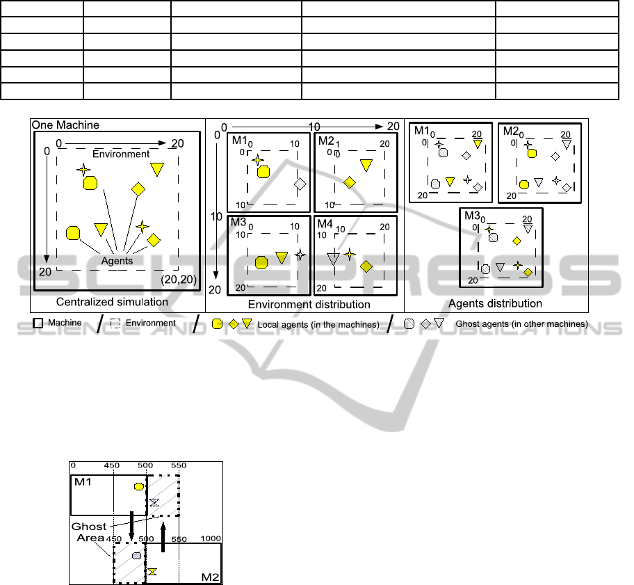
Table 1: Comparison between platforms.
Platform NbOfAgents NbOfMachines Model Distribution types
Repast
68 billions HPC-32000 cores Triangles (simple) Only one type
DMASON
10 millions 64 Boids (simple) Only one type
AglobeX
6500 6 (22 cores) Airplanes (simple) Only one type
GOLEM
5000 50 Packet-World (complex) Only one type
Our testbed 100 millions 200 Prey-predator (more complex) Two types
Figure 1: A centralized simulation can be distributed by two different ways: Environment Distribution or Agent Distribution.
chine has to receive ghost-areas from neighbours and
also has to send ghost-areas for others too. Ghost
area approach is similar to ghost data which is used
with some researchers for visualize parallel simula-
tion (Isenburg et al., 2010).
Figure 2: Exchange information between two machines for
ghost areas (each machine has a surrounding ghost-area
from others).
4 DISTRIBUTED SIMULATOR
DYNAMIC
We focus in this paper on two distribution types: the
environment distribution and the agents distribution.
To implement these two distribution types, we have
developed a prototype with the Java language. The
user can choose which type of distribution he wants
according to his application. In our framework, ma-
chines run with a simple broadcast communication
layer, where each machine can reach other machines.
Each machine makes a part of the calculation during
each time step (TS) and it communicates with others
to build a complete global simulation view. More pre-
cisely, our framework is divided into simulation parts,
each simulation part manages one environment part
with its agents in case of environment distribution or
manage a list of agents in case of agents distribution
(figure 1). Each simulation part consists of three lay-
ers: a communication layer that establishes connec-
tions with others and it is responsible for exchange
messages, a simulator layer that shares information
and transfers agents and an application layer where
agents are defined and are able to interact with each
others. In each time step (TS), the simulator gather all
interactions that agents wish to execute, then analyses
that no conflicting interactions happens (otherwise, a
tie-break rule defines which interaction succeeds and
which one fails) and apply all interactions. Then, the
simulator has to wait for notifications from other ma-
chines before going to the next TS.
The simulation is divided in two main stages, the
initialization stage and the running stage:
• initialization: with environment distribution, the
first step is to divide the environment into dif-
ferent slices on different machines. That can be
through a configurationfile containing lines with a
machine ID, the machine name or IP, the environ-
ment slice ranges and the initial agents contained
within that slice. In case of agents distribution, the
user divide agents between machines in the con-
ICAART2014-InternationalConferenceonAgentsandArtificialIntelligence
314
Environment distribution file:
line1:
EnvironmentDistribution WITHGUI SYNC WITHLOGFILE ...
line2:
ID=0 m1 0 0 10 10 #NbAgent1=50 #Type1=wolf #Nb2 #Type2 ...
line3:
ID=1 m2 10 0 20 10 50 wolf 2000 sheep 3000 grass
line4:
ID=2 m3 0 10 10 20 50 wolf 2000 sheep 3000 grass
line4:
ID=3 m4 10 10 20 20 50 wolf 2000 sheep 3000 grass
Agent distribution file:
line1:
AgentDistribution WITHGUI SYNC WITHOUTLOGFILE ...
line2:
ID=0 m1 0 0 20 20 #NbAgent1=50 #Type1=wolf #NbAgent2 #Type2 ...
line3:
ID=1 m2 0 0 20 20 50 wolf 2000 sheep 3000 grass
line4:
ID=2 m3 0 0 20 20 50 wolf 2000 sheep 3000 grass
Figure 3: An example of configuration txt-files according to the figure 1.
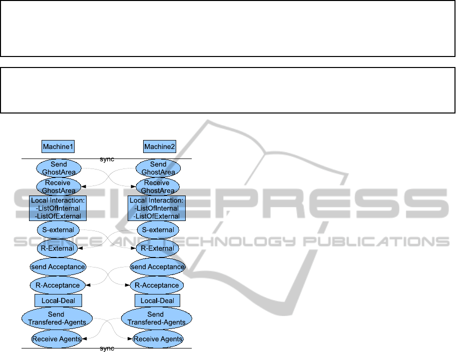
Figure 4: Decomposition of a time step (TS) execution.
figuration file (see figure 3).
• running: during execution, each machine has to
collect information from neighbouring machines
about ghost-area information in case of envi-
ronment distribution or information about other
agents in case of agents distribution. Then, the
simulator asks each agent about its next interac-
tion. However, and in case of environment distri-
bution, if there are agents that cross an edge-zone,
they have to be transferred to another computing
machine. In case of agents distribution, there is
no agent mobility between machines, unless some
load-balancing has to be done.
To be more precise about the dynamic of a simu-
lation step, figure 4 illustrates the main loop that are
applied in the context of two machines.
We first describe all steps for the environment dis-
tribution approach (as illustrated in figure 4), then we
briefly address what is different for agents distribu-
tion:
• Each machine sends its ghost areas to neighbour-
ing machines.
• Each machine waits to receive ghost areas from
its neighbours.
• Each simulator within each machine gathers in-
teractions from its agents and creates two lists:
internal interactions list (between agents on the
same machine) and external interactions list (be-
tween agents that exist on different machines). In-
ternal interactions could be evaluated directly by
the simulator, while external interactions cannot
be evaluated directly because they require some
communication to reach an agreement with other
machines in order to avoid conflicting interactions
(when two wolves want to eat the same sheep for
example).
• Each machine sends its external interactions to
other related machines and waits for agreements
or rejections of interactions. If an interaction is
refused, agents can re-ask for other interactions.
However, it can be implemented as a loop be-
tween machines until all agents are satisfied (all
machines agrees). Normally, it could not be more
than 2 or 3 messages loop that can be exchanged
between machines, but to avoid this loop we sim-
ply drop the interaction if it is refused in this time
step of the simulation.
• After that, all interactions have been resolved and
each machine executes its interactions.
• Then, each machine checks if some agents have to
be moved outside of their environment slice and
if it is the case, theses agents are transferred to
neighbouring machines.
• Finally, all machines are ready to visualize their
environment slices and wait for the synchroniza-
tion barrier before moving to next TS.
In the agent distribution context, the steps are sim-
ilar, but instead of exchanging ghost area informa-
tion, the information about agents that are sent and
EffectiveDistributionofLargeScaleSituatedAgent-basedSimulations
315

Figure 5: Five million agents on 50 machines.
no agent transfer occurs (unless some load-balancing
is taken into account).
Figure 5 shows our testbed scalability with 50
machines to simulate the flocking birds behaviour
(Reynolds, 1999). Each machine has 100000 agents
and the simulation has 50 x 100000 = 5 million agents
in total.
5 EXPERIMENTATIONS
This section details experimentations that have been
realized in order to evaluate our platform scaling. Two
applications have been studied: prey predator (Wilen-
sky, 1997) and a flocking models (Reynolds, 1999).
Prey Predator: which is a classical MAS simulation
using agents with goals. A predator is an organism
that eats another organism (the prey). For example of
predator and prey, we can simulate the co-evolution
of wolves and sheep. Predators and preys evolve to-
gether, the prey is a part of the predator’s environ-
ment, and the predator dies if it does not get enough
food (prey). Also, the predator is a part of the prey’s
environment, and the prey dies if it is eaten by the
predator. The fastest predators in the environment are
able to catch food and eat, so they survive and repro-
duce, and make up more and more of the population.
The fastest preys are able to escape from predators,
so they survive and reproduce, and make up more and
more of the population. An example of this model is
wolf-sheep-grass model (Wilensky, 1997).
Flocking. This simulation illustrates a steer-
ing behaviour that commonly observed with birds
(Reynolds, 1999) (or fish) that evolves in groups. In
this model there is only one kind of agent (like bird)
which can move forward with a group of other near
birds, which are in its perception range. Normally
in this simulation and after some iterations, groups
of agents are emerging and after some times, there
is only one big group of birds that moves smoothly
together. On the environment’s view, there is non ho-
mogeneous distributions, some parts of the sky hold a
lot of birds, while others are less filled.
These applications have been chosen because they
imply distinct population dynamics. Indeed, in a prey
predator model, prey and predator are moving but
they are homogeneously distributed within the envi-
ronment, while the flocking model, even if the distri-
bution is homogeneous at the beginning of the sim-
ulation, rapidly flocks emerge and after some times,
only one main flock appears. It means that these two
applications illustrate the trade-offthat has to be made
while distributing the load across a computer network,
and the type of distribution can give really different
results.
5.1 Experimentations Description
All the following experiments have been done on ho-
mogeneous hardware with a basic Linux PCs network
(Intel-R CoreTM2 Duo CPU E8400 3.00GHz, mem-
ory 4GB and 100Mb connection). In these experi-
ments, several initial configurations have been set:
• We are able to simulate a large-scale experiments
on 50 machines with 5 million agents (see figure
5). But to facilitate the performance measuring,
some experiments are ranging from 1 up to 16 ma-
chines.
• At the beginning of the simulation, the number of
agents which is usually used: for prey-predator
(Wolf-Sheep-Grass model) 5000 agents per ma-
chine, for flocking (Birds) 10000 Agents per ma-
chines. That means, if we have one experience
with 2, 4, 8 and 16 machines, we use 5000x16 =
80000 agents for 16, 8, 4 and 2 machines to
make a reasonable comparison between machines
in this experimentation.
• For the agent distribution list, agents are divided
equally between machines.
• For the environment distribution, environment are
divided equally between machines as a grid as
possible (see figure 1).
• Perceptions of all agents are small with respect
to the environment slices that are used, and the
size of ghost areas has been chosen as the max-
imum agent perception to avoid any privation of
any agent.
5.2 Scaling the Platform from 9 to 50
Machines
We have tested a wolf-sheep-grass model with initial
250000 agents distributed on 9, 16, 25 and 50 ma-
ICAART2014-InternationalConferenceonAgentsandArtificialIntelligence
316
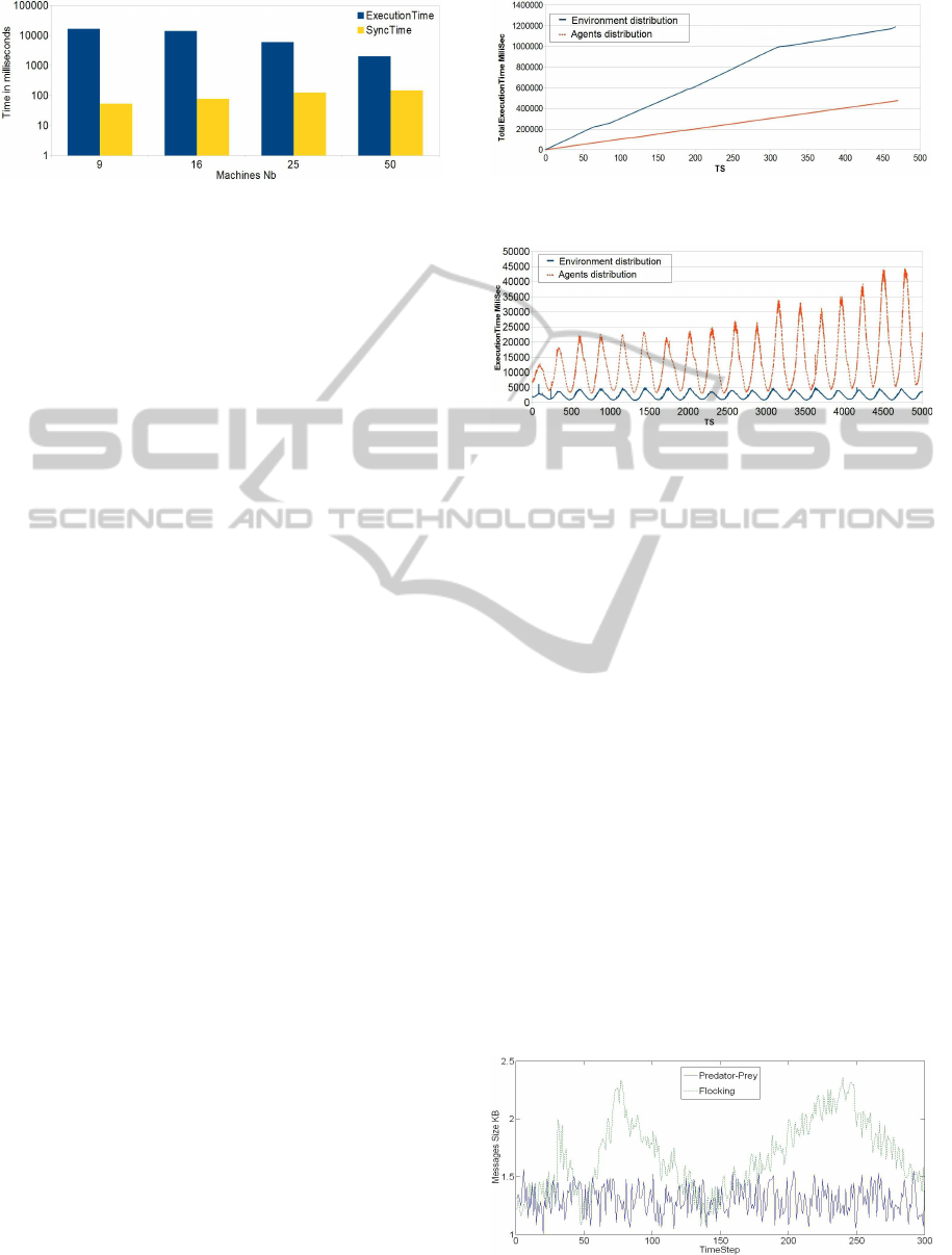
Figure 6: TS delay & communication delay in prey-predator
model with environment distribution approach.
chines by environment distribution approach. Figure
6 shows that the execution time is significantly re-
duced when more machines are used. In this figure,
the first column represents the whole execution time,
while the second one is the synchronization delay.
The figure shows that with small number of machines,
the synchronization delay is small and the execution
time is large as the number of agents is large too.
Whereas, if the number of agents small and the num-
ber of machines is larger (in case of 50 machines),
the synchronization delay has to be large too, but the
execution time is small. It is clear that, it will not
be efficient to distribute small number of agents on
large number of machines or large number of agents
on small number of machines.
5.3 Effective Distribution of a MAS
Simulation
Next experiments evaluate the performance of our
distributed simulation with two types of distribution:
environment distribution and agents distribution, and
on two models: Flocking and prey-predator.
Figures 7 and 8 show results for two types of dis-
tributions (agents and environment) for each appli-
cations. Figure 7 shows that in flocking model and
in case of agents distribution the performance is bet-
ter than environment distribution. That is because,
in case of environment distribution there are huge
groupsof birds that can fly together and swap between
machines. That can increase the execution time as
there are more charge of birds on one machine (one
environment part) than others. Whereas, in case of
agent distribution we have the same number of agents
on each machine and the execution time will be the
same for all. Figure 8 shows that prey-predator model
has completely opposite action than flocking model,
the execution time is better in case of environment
distribution type than agent one, that is because there
are no huge groups of agents on the same patch of en-
vironment and swap between machines (like the case
of flocking). In prey-predator model, agents can re-
produce and die during the simulation time steps, for
Figure 7: Total execution-time of flocking model with two
different distribution types.
Figure 8: Execution-Time of prey-predator model with two
different distribution types.
that the execution time looks like a cosine function
as the number of agents is reduced and re-increased
during the simulation.
To summarize, environment distribution type is
better for prey-predator model than agents distribu-
tion one, whereas agents distribution type is better for
flocking model than environment one.
5.4 Communication Costs Evaluation
In this experimentation, we evaluate the volume of
messages exchanged in our two applications. We test
the flocking and wolf-sheep-grass models on two ma-
chines with environment distribution approach. Fig-
ure 9 shows that the flocking model has important
variations in messages volume, while prey-predator
model did not have such peaks and is more stable.
These differences come from the agent behaviour:
in flocking model, we may have a huge number of
birds moving from one machine to another and that
means bigger messages to transfer these agents and so
more communication costs. Whereas in prey-predator
Figure 9: Communication costs of 300 TS in environment
distribution approach.
EffectiveDistributionofLargeScaleSituatedAgent-basedSimulations
317
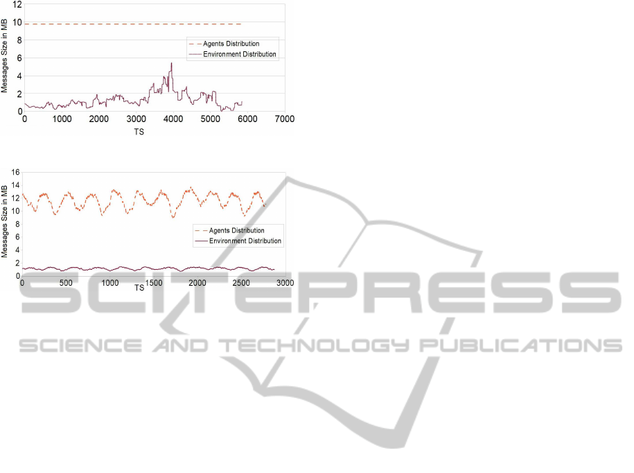
Figure 10: Messages size of flocking simulation.
Figure 11: Messages size of prey-predator simulation.
model, it is not the case because agents do not have
group behaviours like in the flocking, so the model
is more stable in messages exchanged between ma-
chines. This figure demonstrates that in distributed
multi-agents simulations with spatial environments,
speed up is highly related to the dynamic of agents
movements and agents models.
To detail more flocking behaviour, we test com-
munication cost on both distribution types, figure 10
shows that the communication cost is large in agents
distribution type than environment one but more sta-
ble. That is because in flocking with agent distribu-
tion, the number of agents fixed in all machines and
the information which has to be sent between ma-
chines should be in the same size too. Whereas in
environment distribution, some of the birds can be to-
gether in one big group on the sky (on one machine),
and other machines maybe have less birds. That
should make the communication cost is lower but less
stable (variant) in environment distribution. However
in prey-predator model (figure 11), the stability exists
in environment distribution and not in agent distribu-
tion, that is because in prey-predator model there are
agents that reproduce and die during the simulation
time steps in the same machines. Thus in agent dis-
tribution, it can make more (or less) charge of agents
in one machine than others, and messages size can be
changed during the simulation to look like a cosine
function (as the number of agents is reduced and re-
increased during the simulation) that can make it less
stable in agent distribution than environment one.
5.5 When Should We Use Each Type of
Distributions
Table 2 shows a comparison between the two mod-
els (prey-predator and flocking) with two distribu-
tion types (agent and environment). Environment dis-
tribution type is better in execution time for prey-
predator model than flocking model, whereas agents
distribution type is better for flocking model than
prey-predator model. However, for communication
costs, environment distribution is more stable for
prey-predator model than agent distribution, whereas
agents distribution is more stable for flocking model
than environment one. To summarize, some distri-
bution types are more suitable for some applications
than others.
To analyse this result, we try to extract some gen-
eral features from both models, then the user can
choose which distribution type is more suitable for
his application (see table 3). In prey-predator model,
agents’ life-cycle is short (N TS) and agents exist
overall the environment. Whereas in flocking model,
it is completely opposite to that, agents’ life-cycle is
long and agents may be aggregated during the simu-
lation in one place only (not everywhere). The aggre-
gation and the long life-cycle could make the environ-
ment distribution approach is bad solution for flock-
ing model, because computation can be aggregated in
one machine only. For that, the agents distribution
is the best solution for flocking model. Whereas for
prey-predator, it is completely inverted.
6 CONCLUSIONS
In this paper, we have proposed two types of distri-
bution for multi-agent systems: environment distri-
bution and agents distribution. We have evaluated it
with two different applications, which are the flocking
behaviour in birds and prey-predator models. In case
of environment distribution, the simulated environ-
ment is divided into different partitions on different
machines (each partition is allocated on one machine
only). During the simulation, each machine commu-
nicates with its neighbouring machines to collect a
needed information about common areas (or ghost-
area). In case of agents distribution, the simulated en-
vironment is the same for all machines and agents will
be divided between machines. During the simulation,
each machine communicates with others for collect-
ing needed information about other agents (or ghost-
agents) which exist on other machines. We propose
a simple protocol to allow all machines from com-
municate between each other to build a distributed
ICAART2014-InternationalConferenceonAgentsandArtificialIntelligence
318
Table 2: A comparison between two models with two distribution types.
Model Agent distribution Environment distribution
Prey-predator execution time Not efficient Efficient
Flocking execution time Efficient Not efficient
Prey-predator communication cost Not stable Stable
Flocking communication cost Stable Not stable
multi-agent simulation. The main technical prob-
lem to resolve was interactions between two agents
or more from different machines, which is solved by
an agreement protocol. Experimental results show
that the proposed distribution types have better per-
formances in some models than others. For example,
prey-predator model has better performance in the ex-
ecution time than flocking model when we distribute
the environment. Whereas, agents distribution type is
better for flocking model. The current implementa-
tion provides a good framework for future works, we
plan to investigate more the two types of distributions,
and try to implement a hybrid approach, which maybe
give us better performance in most models. We plan
to increase the scalability of our framework. We cur-
rently reach near 5 million agents and we plan to dis-
tribute multi-billions agents in less than one minute
for one simulation time step.
Table 3: Analysis of agent’s features between two models:
prey-predator and flocking.
Agent Features Prey-predator Flocking
Life-cycle Short Long
Movement Small area Large area
Positioning Everywhere Aggregation
Reproducing Exist Not exist
REFERENCES
Bromuri, S. and Stathis, K. (2009). Distributed agent en-
vironments in the ambient event calculus. In Proc.of
DEBS, pages 12:1–12:12, New York, USA. ACM.
Cordasco, G., Rosario, D. C., Ada, M., Dario, M., Vitto-
rio, S., and Carmine, S. (2011). A framework for
distributing agent-based simulations. In Proc. of Het-
eroPar2011. Springer Berlin Heidelberg.
Cosenza, B., Cordasco, G., De Chiara, R., and Scarano, V.
(2011). Distributed load balancing for parallel agent-
based simulations. In PDP.
Isenburg, M., Lindstrom, P., and Childs, H. (2010). Parallel
and streaming generation of ghost data for structured
grids. CGA, IEEE, 30(3):32 –44.
Jefferson, D. R. (1985). Virtual time. ACM Trans. Program.
Lang. Syst., 7:404–425.
Kuhl, F., Weatherly, R., and Dahmann, J. (1999). Creating
computer simulation systems: an introduction to the
high level architecture. Prentice Hall PTR, NJ, USA.
Logan, B. and Theodoropoulos, G. (2001). The distributed
simulation of multiagent systems. Proceedings of the
IEEE, 89(2):174 –185.
Miyata, N. and Ishida, T. (2008). Community-based load
balancing for massively multi-agent systems. In
Massively Multi-Agent Technology, volume 5043 of
LNCS, pages 28–42. Springer Berlin / Heidelberg.
Motshegwa, T. and Schroeder, M. (2004). Interaction mon-
itoring and termination detection for agent societies:
Preliminary results. In ESAW, volume 3071 of LNCS,
pages 519–519. Springer Berlin / Heidelberg.
Reynolds, C. (1999). Steering behaviors for autonomous
characters.
Russell, S. J. and Norvig, P. (1996). Artificial intelligence:
a modern approach. Prentice-Hall.
Scerri, D., Drogoul, A., Hickmott, S., and Padgham, L.
(2010). An architecture for modular distributed sim-
ulation with agent-based models. In AAMAS’10 Pro-
ceedings., pages 541–548.
Siebert, J., Ciarletta, L., and Chevrier, V. (2010). Agents
and artefacts for multiple models co-evolution: build-
ing complex system simulation as a set of interacting
models. In Proceedings of the 9th Int. Conf. on AAMS,
AAMAS ’10, pages 509–516, Richland, SC. IFAA-
MAS.
ˇ
Siˇsl´ak, D., Volf, P., Jakob, M., and Pˇechouˇcek, M. (2009).
Distributed platform for large-scale agent-based sim-
ulations. In Agents for Games and Simulations, pages
16–32. Springer-Verlag, Berlin.
Wilensky, U. (1997). Netlogo wolf-sheep predation model.
Wooldridge, M. and Jennings, N. R. (1995). Intelligent
agents: theory and practice. The Knowledge Engi-
neering Review, 10:115–152.
Yamamoto, G., Tai, H., and Mizuta, H. (2008). A plat-
form for massive agent-based simulation and its eval-
uation. In Jamali, N., Scerri, P., and Sugawara, T.,
editors, Massively Multi-Agent Technology, volume
5043, pages 1–12. Springer Berlin Heidelberg.
EffectiveDistributionofLargeScaleSituatedAgent-basedSimulations
319
