Synthesis and Abstraction of Constraint Models for Hierarchical

Resource Allocation Problems

Alexander Schiendorfer, Jan-Philipp Stegh

ofer and Wolfgang Reif

Institute of Software & Systems Engineering, Augsburg University, Augsburg, Germany

Keywords:

Hierarchical Resource Allocation, Constraint Satisfaction Problems, Model Abstraction, Autonomous Power

Management.

Abstract:

Many resource allocation problems are hard to solve even with state-of-the-art constraint optimisation software

upon reaching a certain scale. Our approach to deal with this increasing complexity is to employ a hierarchical

“regio-central” mechanism. It requires two techniques: (1) the synthesis of several models of agents providing

a certain resource into a centrally and efﬁciently solvable optimisation problem and (2) the creation of an

abstracted version of this centralised model that reduces its complexity when passing it on to higher layers. We

present algorithms to create such synthesised and abstracted models in a fully automated way and demonstrate

empirically that the obtained solutions are comparable to central solutions but scale better in an example taken

from energy management.

1 INTRODUCTION

Resource allocation problems present themselves in a

variety of domains (Chevaleyre et al., 2006), includ-

ing autonomous power management (Anders et al.,

2013b) or grid computing (Abouelela and El-Darieby,

2012). Constraint programming provides a wide

range of algorithms and techniques targeted at solv-

ing and optimising problems including resource al-

location that are readily available in state-of-the-art

software. By virtue of this general formalism for stat-

ing problems declaratively in terms of variables, do-

mains, and constraints, many different problem in-

stances can be tackled with these algorithms. This

proves particularly useful when the characteristics of

heterogeneous agents need to be modelled. If, how-

ever, the size of the system prohibits a centralised so-

lution, due either to the communication overhead re-

quired in collecting all necessary information or due

to the complexity of a centralised solution model, hi-

erarchical decomposition provides a generic approach

to deal with these issues (see, e.g., Abouelela and

El-Darieby, 2012; Boudjadar et al., 2013). In such

cases, distributed, cooperative, agent-based systems

can be employed in which the agents form organisa-

tions. The global problem is hierarchically decom-

posed and the organisations collaboratively and recur-

sively solve a sub-problem. The overall solution is the

combination of the sub-solutions. It is not necessarily

globally optimal, since each organisation works with

regional knowledge only, but the scalability beneﬁts

often outweigh this drawback.

Decisions in such problems depend on the capa-

bilities of the individual components on the lowest

level. To make correct decisions further up in the

hierarchy, this information must at least be partially

propagated to these higher levels. Since hierarchical

solving is employed in cases where the scale of the

system prohibits a fully centralised solution, informa-

tion must be abstracted when propagated upwards or

the scalability beneﬁt will be lost. At the same time,

the information provided by the distinct agents on the

lower hierarchy levels must be synthesised to gain a

solvable model.

While fully decentralised approaches (Yokoo

et al., 1998) deal with the scalability problem as well,

they work with even more limitations on the infor-

mation available and introduce communication over-

head. The hierarchical or regio-central approach cen-

tralises information from a region of the system and

solves this sub-problem centrally. Depending on the

hierarchical structure of the system, many such re-

gions can exist and they all solve the sub-problems

concurrently as shown with examples in Section 3.

Resource allocation problems and their hierarchi-

cal specialisation can be expressed as constraint satis-

faction and optimization problems (also referred to as

constraint models) to make use of highly optimised

Schiendorfer A., Steghöfer J. and Reif W..

Synthesis and Abstraction of Constraint Models for Hierarchical Resource Allocation Problems.

DOI: 10.5220/0004757700150027

In Proceedings of the 6th International Conference on Agents and Artiﬁcial Intelligence (ICAART-2014), pages 15-27

ISBN: 978-989-758-016-1

 2014 SCITEPRESS (Science and Technology Publications, Lda.)

general purpose constraint solvers (see, e.g., Hladik

et al., 2008; Santos et al., 2002). Our synthesis and

abstraction approach assumes that the models of con-

crete producer agents are available as constraint mod-

els. This paper introduces two techniques for using

constraint models in a hierarchical setting:

Synthesis: the models provided on a lower level

are combined and augmented with organisation-

speciﬁc constraints to form an optimization prob-

lem that can be solved in a regio-central way. The

solution of this model is distributed to the agents

on the lower level.

Abstraction: the information contained in the mod-

els of one region is abstracted to form a new

model of the hierarchy level which is then pro-

vided to the next higher level. In this way, higher

levels are not overwhelmed with the details of the

lower levels but can still provide solutions that

can actually be achieved by the lower levels. Our

understanding of abstraction follows Giunchiglia

and Walsh (1992): “Abstraction is the mapping of

a problem representation into a simpler one that

satisﬁes some desirable properties in order to re-

duce the complexity of reasoning.”

There are several reasons to pursue this approach:

First, constraint languages offer ﬂexibility suitable

for organisations of heterogeneous agents and prob-

lems and can be solved with established algorithms.

Second, a large problem instance is broken into

smaller subproblems (fewer decision variables and

constraints) which tend to be easier to solve to offer

scalability. And lastly, individual agent models can

be crafted without taking others into account and sev-

eral agent models are automatically combined to be

solved regio-centrally which allows for fast recom-

bination and reduces communication overhead com-

pared to a fully distributed solution.

We will detail the lifecycle and algorithms for

this regio-central solution approach with a case study

from autonomous power management. The goal is

to ﬁnd “schedules” for controllable power plants, i.e.,

instructions of how much power they have to produce

at which point in time, based on the predicted demand

and the predicted input of weather-dependent power

plants at that time. The details of this case study will

be explained in Section 3.

Related Work. The term “model abstraction” was

coined by the simulation engineering community and

Frantz (1995) provides a taxonomy of common model

abstraction techniques, some of which are found in

our approach as well such as piecewise linear func-

tions to approximate general functions. As an ex-

ample of work in this area, Lee and Fishwick (1996)

used neural networks to get a behavioural abstraction

of subcomponents that were given as state machines.

Their goal was to run simulations on different lev-

els independently of lower levels — which is simi-

lar to solving constraint problems based on abstrac-

tions. Pelikan and Goldberg (2000) found hierarchi-

cal decomposition to be useful in genetic algorithms

by combining solutions from lower levels to solu-

tions on higher levels similar to the presented method.

While they also made a case for hierarchical problem

solving in general, they put emphasis on how to im-

prove existing genetic and evolutionary algorithms.

Our method works with any existing constraint op-

timization algorithm but is designed for a particular

problem class. Kinnebrew and Biswas (2009) devel-

oped a hierarchical variant of the contract net protocol

that also offered scalability beneﬁts. Choueiry et al.

(1994) presented abstraction methods for task and re-

source allocation problems and focussed on heuris-

tics that ﬁnd interchangeable sets of tasks but did not

emphasise production processes. The approach pre-

sented in this paper depends on an interval representa-

tion and does not cover tasks that share resources but

rather deals with resource allocation problems with-

out side effects, as described in Section 2.

Our method combines techniques from traditional

model abstraction from the simulation domain with

constraint programming to solve hierarchical resource

allocation problems. To the best of our knowledge,

this is a novel approach with promising ﬁrst results as

will be outlined in Section 6.

2 HIERARCHICAL RESOURCE

ALLOCATION PROBLEMS

We ﬁrst present the abstract structure of the problems

our approach is applicable to and then show how the

load balancing problem in autonomous power plant

management is an example of this problem class. All

problems we consider are representatives of the gen-

eral one-good resource allocation problem without

externalities (Van Zandt, 1995): Given a total quan-

tity x

of a resource, ﬁnd an allocation hx

,...,x

i of

the resource to n agents to solve

minimise

,...,x

∑

i=1

) subject to

∑

i=1

= x

where c

) is a cost function for allocating x

of the

resource to agent i. Since this problem is stated to

have no externalities and thus allocations do not have

side effects on other agents, it can be decomposed into

similar independent sub-problems. Therefore, agents

ICAART2014-InternationalConferenceonAgentsandArtificialIntelligence

can be combined in hierarchical organizations. Allo-

cating resources ﬁrst to organisations of agents and

then distributing the resources within the organisa-

tions solves the overall problem.

The problems covered by our approach take into

account additional aspects: In our setting, the ultimate

problem consists of allocating the production of some

resource to a set of agents such that a given (possibly

predicted) demand is met by the combined production

over a given time range as well or as cost-effectively

as possible. Since meeting this demand is not always

feasible, we encode the deviation of demand and pro-

duction as the cost function to be optimised as op-

posed to stating it as a hard constraint. The possible

contributions of a single agent are however limited to

certain ranges that can include no production at all.

Additionally the allocation in earlier time steps affects

future possible allocations. An allocation of resources

over some time range will be referred to as schedule.

More formally, let A be a set of agents where the

possible contributions to the total demand is given by

for each a ∈ A , an ordered list of non-overlapping

intervals ∈ R

. An agent can be excluded from the

combined allocation if and only if 0 is covered by

some interval. Indeed, the choice of lists of intervals

is motivated by the fact that practical problems may

enforce minimal and maximal economical boundaries

if any contribution is made. But agents can also be

excluded entirely from production. Allocations are

created for a ﬁnite time range T from 1 to some up-

per bound max(T ). Similarly, the demand that has to

be satisﬁed is given by D

∈ R, t ∈ T . The produc-

tion assigned to some agent a in time step t is denoted

by P

. A state Σ

∈ Σ, t ∈ T , a ∈ A is a set of vari-

ables that contains all information available to a pro-

ducer a up to some time step t that is required to make

decisions over the production in the next time step

t + 1. In particular, Σ

contains P

for all t

∈ 1, . . . ,t,

hence the complete run up to t. Additionally, other

variables such as the number of time steps an agent

did not contribute can be part of Σ

as they might be

needed for speciﬁc constraints such as startup times

for agents. Some constraints employ a pair of func-

tions, c

min

max

: Σ → R, that restrict the possible al-

locations in the next step based on the current state.

These considerations yield a core optimization

model that needs to be solved:

minimise

∑

t∈T

−

∑

a∈A

subject to ∃[x,y] ∈ L

: x ≤ P

≤ y, ∀a ∈ A, t ∈ T

t+1

≥ c

min

(Σ

), ∀a ∈ A, t ∈ T

t+1

≤ c

max

(Σ

),∀a ∈ A, t ∈ T

Abstraction

Synthesis

IAM

SRM

AAM

Synthesis

IAM

SRM

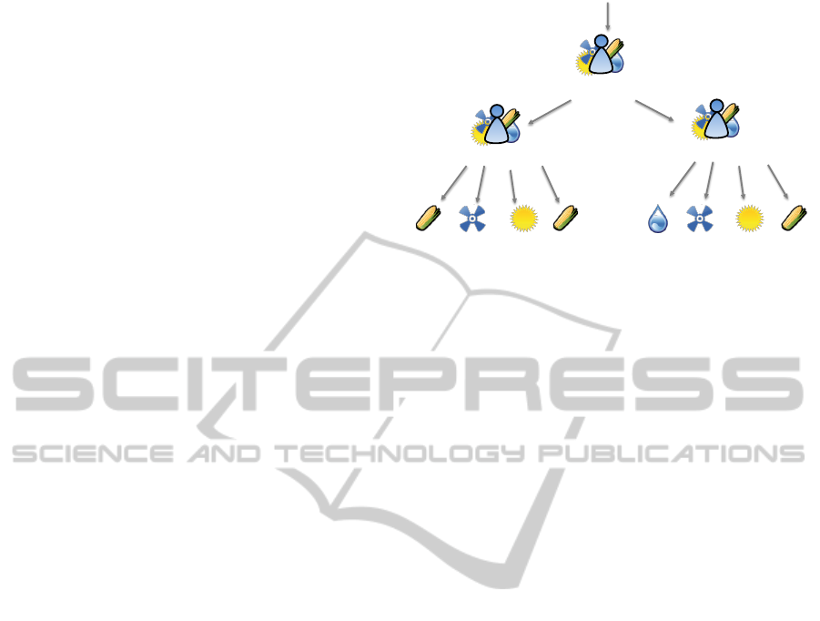
Figure 1: A sample hierarchy of power plants providing.

Bold font indicates model types, arrows represent transfor-

mations between them.

Several agents can be combined to form a new

agent that manages the production of its subordinates

representing an organisation. As this agent is not a

physical producer itself that introduces new possible

contributions but rather combines existing agents we

refer to it as a virtual agent (VA). An agent hierar-

chy H formally is a tree of agents and virtual agents

where for some virtual agent v, children(v) represents

the child nodes of v and a ∈ children(v) holds iff

parent(a) = v. A virtual agent, more precisely, the set

of all its child nodes is also referred to as “region”.

The general algorithm solves the hierarchical re-

source allocation problem in a top-down fashion by

ﬁrst distributing the demand among the children of

the root agent using a constraint solver and then have

the children recursively solve their allocation problem

until all leaf nodes are assigned some amount of the

resource as Figure 2 shows. In light of this algorithm,

the purpose and necessity of synthesis and abstrac-

tion become clear. Synthesis creates an optimization

problem based on models of concrete agents and ab-

straction leads to a simpliﬁed model used for a vir-

tual agent on higher levels. Contrary to the demand

distribution, model synthesis and abstraction are thus

bottom-up algorithms.

There are three different types of models involved

in our approach. The ﬁrst two model types represent

a mathematical description of the agents’ underlying

physical systems whereas the last model puts these in

an optimisation context. The rationale is to separate

the task of modelling a system from formulating an

optimisation problem. Figure 1 depicts the relation-

ships of models in synthesis and abstraction:

Individual Agent Models (IAM) describe the prop-

erties of one concrete agent representing a physi-

cal entity in terms of constraints for the available

production in T time steps depending on its own

state (being on/off, production levels etc.) regard-

less of other agents. This model needs to be pro-

vided by an agent designer. An IAM deﬁnes the

feasible production intervals of an agent but also

regulates possible transitions between production

levels at different time steps.

SynthesisandAbstractionofConstraintModelsforHierarchicalResourceAllocationProblems

Abstracted Agent Models (AAM) are simpliﬁed

agent models of a set of underlying agents that

capture the essentials and serve as models of

virtual agents that can be given to a superior

instance. To this higher instance, it does not

matter whether it is confronted with an individual

agent or an already abstracted model.

Synthesised Regional Models (SRM) combine sev-

eral agent models to yield the regio-central con-

straint models which describe the resource allo-

cation problem within a virtual agent. The com-

bined production is the sum of all subordinate pro-

ductions. Additionally, constraints such as “pre-

fer agents of type X” or “distribute residual load

evenly” can be stated here. These types of mod-

els include both the actual load distribution opti-

mization problem as well as the models used in

sampling abstraction. Since preferences or soft

constraints can be stated in addition to hard con-

straints, the resulting problems are instances of

soft constraint models (Meseguer et al., 2006).

Let AM be the set of agent models such that

AM = IAM ∪ AAM and SRM ⊂ SCSP the set of soft

constraint satisfaction or optimization problems that

model a region. We can then ﬁrst deﬁne the synthesis

and abstraction processes:

synth : 2

→ SRM

abstract : 2

→ AM

Hence, synthesis creates an optimization problem for

resource allocation based on the formal models of a

set of agent models. Abstraction creates another agent

model from a set of agent models representing the un-

derlying agents. We will describe the contents of the

synth and abstract procedures in the following sec-

tions but ﬁrst show concrete problem instances.

3 INSTANCES OF

HIERARCHICAL RESOURCE

ALLOCATION

To illustrate our approach, we present two concrete

instances of hierarchical resource allocation prob-

lems. Our case study is taken from distributed energy

management systems. To illustrate the generality of

our approach, we additionally show a load balancing

problem in server clusters in our framework.

Organization

Top-Level-

AVPP

50K kWh

30K kWh

20K kWh

10K

5K 10K

15K

0K 3K

Figure 2: An exemplary AVPP structure. AVPPs can con-

tain other AVPPs. Leaf nodes indicate different types of

power plants (e.g., wind, solar, biomass, running water).

Edges indicate how the incoming load is distributed.

3.1 Hierarchical Power Plant

Scheduling

Future energy management systems require ﬂexible

resource allocation mechanisms. Or, as Ramchurn

et al. (2012) put it: “It will be important to design de-

centralised coordination algorithms and strategies that

allow individual [. . . ] participants to come to the most

efﬁcient arrangements within a reasonable time.” One

of the most prominent tasks is to control power plants

in a way that balances production and demand. In par-

ticular, these two quantities need to be in approximate

equilibrium as to keep the mains power frequency in a

small corridor to achieve stable power supply (Heuck

et al., 2010). The output of power generators needs

to be controlled in accordance to the predicted con-

sumption. However, the problem of load balancing

in energy systems is known to be an NP-hard prob-

lem in general (Bar-Noy et al., 2001) and therefore

centralised solutions fail to scale with an increasing

number of controlled plants.

Our approach is based on the notion of Au-

tonomous Virtual Power Plants (AVPPs) (Stegh

ofer

et al., 2013a). Figure 2 shows a typical AVPP struc-

ture which embodies a control scheme for the load

distribution in the context of a self-organizing sys-

tem. An AVPP takes the role of a virtual agent re-

sponsible for a set of subordinate power plants and

can itself be controlled in a hierarchy. Each AVPP

is responsible for satisfying a fraction of the over-

all demand. Its structure changes in response to new

information and changing conditions to enable each

AVPP to balance its power demand and production

(consequently forming the hierarchy as described in

Stegh

ofer et al., 2013b) — thus fast recombination

is desirable. Each AVPP calculates schedules that

manage the output of its assigned controllable power

plants for future points in time and therefore also its

ICAART2014-InternationalConferenceonAgentsandArtificialIntelligence

own output. AVPPs need to rely on predictions about

the future demand as well as the future output of non-

controllable power plants to approximate the residual

load (i.e., the consumption minus the production sup-

plied by non-controllable plants) which has to be met

by controllable power stations. Arising uncertainties

are dealt with by means of robust optimization meth-

ods using trust-based scenarios as described in (An-

ders et al., 2013a).

In the context of power management, the resource

is electric power and we refer to an allocation of the

residual load to power plants for some time range

as the schedule. The common optimization prob-

lem structure presented in Section 2 thus applies with

power stations being the agents and AVPPs the virtual

agents. Power plant models need at least to provide

some minimal and maximal power boundaries, P

min

and P

max

since power stations have a lower bound for

economically reasonable production. The predicted

residual load represents the demand. In addition, var-

ious plant-speciﬁc constraints may describe the char-

acteristics of a power station such as a minimal startup

time, minimal running and standing times and, most

prominently, a limited rate of change P

between two

consecutive time steps which may be relative to the

current production or a ﬁxed amount. As we assume

that the agents’ contributions are subject to inertia —

a typical property of power generators — the resource

allocation problem needs to be solved for a future

time frame in advance (Heuck et al., 2010; Anders

et al., 2013b).

3.2 Cluster Load Balancing

Consider the problem of load balancing HTTP re-

quests in a cluster of servers inspired by efforts to

distribute processing capacity in grid applications in-

vestedigated by Abouelela and El-Darieby (2012).

Assume that “masters” are capable of assigning re-

quests to “slaves” that handle the requests. A slave

needs to communicate the minimal and maximal

number of requests it may process at one time step

to its master — minimal requests are useful to justify

the communication overload associated with employ-

ing a machine. The masters are organised hierarchi-

cally, where one master needs to represent the capa-

bilities of its subordinate slaves or masters and a top

level master receives the incoming requests. Upon de-

ciding what number of requests the slaves receive to

process, actual requests are distributed. Note that we

do not argue that this approach is the most efﬁcient

way to solve this problem but rather shows another

possible application of model synthesis and abstrac-

tion.

The set A consists of the slaves and masters,

where the latter represent virtual agents that are or-

ganised in a given hierarchy. The production P

rep-

resents the number of requests handled by agent a in

time step t as a natural number. In this model, the

states Σ

track the requests currently processed to pre-

dict how many requests can be taken in step t + 1.

4 SYNTHESIS OF

REGIO-CENTRAL MODELS

Aside from the generally required parameters of the

individual agent models introduced in Section 2 such

as the possible contributions of agents, the constraint

models can exhibit varying characteristics regarding

feasible schedules. These may take the form of con-

straints that restrict the change in production of an

agent to less than x% between two time steps or that

requires an agent to contribute for a minimum number

of consecutive time steps.

In our approach, we distinguish constraint models

used as declarative formal models of the producing

agents (AM) and models for optimising the resource

allocation problem (SRM). Individual preferences are

formulated as soft constraints and inﬂuence the op-

timisation function. Such preferences could include

that it is better to stay within a subrange of production

for an IAM or that all agents are equally contributing

instead of an extremal distribution for a SRM. They

are speciﬁed as constraint relationships (Schiendorfer

et al., 2013) which, in essence, are a binary relation

over the soft constraints that induce a partial order

over solutions. If no solution for all constraints can

be found, constraint relationships deﬁne which con-

straints are more important to be satisﬁed and encode

this information as weights that serve as penalties for

an optimisation function. Intuitively, more important

constraints receive higher weights so a quantitative

cost function consistent with the induced partial or-

der is created.

An IAM or AAM for an agent a provides a list

of feasible production spaces L

as well as con-

straints that regulate production transitions between

time steps. A SRM for a virtual agent v results from

combining a set of agent models of its children and

is a soft constraint satisfaction problem (SCSP) given

by hX , D, C ,R i for some time range T where

• X are decision variables that take values from

their associated domain D(x), for x ∈ X . In par-

ticular, P

⊆ X , t ∈ T , a ∈ children(v).

• C are constraints that specify which assignments

of values to variables are valid. Constraints can

SynthesisandAbstractionofConstraintModelsforHierarchicalResourceAllocationProblems

either be speciﬁed intensionally (P

≥ 500) or ex-

tensionally (by enumerating valid variable assign-

ments). There exist hard constraints, C

, that are

mandatory and soft constraints, C

, which should

be satisﬁed as well as possible such that C

∪C

C , C

∩ C

0. The constraints stated in AMs are

combined by taking their union since their scopes

do not overlap (each AM constraint regulates as-

signments to variables over time in one agent).

• Constraint Relationships, R ⊂ C

× C

deﬁne a

binary preference relation such that c



iff

is more important than c

. Each agent may

provide such a relation for its soft constraints

such as “optimalRange :(1000 ≤ P

≤ 2000) 

acceptableRange :(500 ≤ P

≤ 2500)” to state its

individual preferences regarding its own contribu-

tion (for the implementation, constraint relation-

ships are transferred into weights such that for

each agent a utility function over solutions can be

constructed – see Schiendorfer et al., 2013).

In addition to taking the union of all variables and

domains of the agent models under renaming to avoid

name clashes when creating the SRM, for a virtual

agent v, a variable P

is added to represent the ac-

cumulated production for each time step t. Consis-

tency is enforced by a hard constraint P

∑

a∈A

where A

are the children of v. The union of all con-

straint relationship sets is taken and possible organi-

sational soft constraints of the SRM (such as “balance

the load assignment”) are deﬁned to be more impor-

tant than the soft constraints of the AMs as organisa-

tional goals such as an even distribution are designed

to be more important than individual preferences. An

optimisation problem is then deﬁned by adding an op-

timisation function f : (X → D) → R. Hence, solu-

tions (assignments satisfying all hard constraints) are

totally ordered. Minimizing the gap between demand

and production is then achieved by using the function

presented in Section 3: minimise

∑

t∈T

− P

|. In-

corporating constraint relationships requires the solu-

tion of a multi-objective optimisation problem, i.e.,

the original objective as well as the violation of soft

constraints have to be optimised. Other objectives

such as cost effectiveness could be encoded. This

synthesised regional model is then used to solve the

actual resource allocation problem with constraint or

mathematical programming algorithms such as mixed

integer programming (MIP).

5 ABSTRACTION OF

REGIO-CENTRAL MODELS

Virtual agents can be regarded as another type of pro-

ducing agent that itself might be controlled. In fact,

every VA other than the top-level VA is managed by

a superior agent. Consequently, this governing VA

also needs a constraint model of its subordinate agents

in order to distribute the demand. Instead of just

merely copying all constraints and decision variables

included in the SRM to higher hierarchy levels (which

would effectively just result in a centralised model)

we introduce some reduction of complexity by an au-

tomated abstraction algorithm. Certainly, abstraction

will cause to errors due to imprecisions but leads to

a scalable resource allocation scheme. We will dis-

cuss possible approaches to construct a valid AAM of

a virtual agent.

Since the AAM should be equivalent to an IAM

in the sense that a superior agent does not need to

bother whether it manages a virtual or concrete agent,

an AAM also deﬁnes possible production ranges and

transitions between productions for P

. Thus, ab-

straction aims to describe the available ranges of pro-

duction of a synthesised model in a compact way and

introduces new constraints representing the relations

of the aggregate of all subordinate agents. We are

interested in ﬁnding the “corners” of the production

space spanned by a VA as well as possible “holes”,

i.e., contributions that can never be produced by a VA

in its current conﬁguration. We propose three differ-

ent kinds of abstraction that result in different con-

straints for P

that can be combined to obtain one ab-

stracted constraint model.

5.1 General Abstraction

A ﬁrst question of interest for abstraction is to ﬁnd

feasible intervals of a VA given the possible produc-

tions of its subordinate agents. As the contribution of

an individual agent may be discontinuous (e.g., when

an agent has a minimal production boundary > 0 but

may also not contribute at all), the possible space of

production is discontinuous in general: Consider a

VA responsible for two agents and the possible con-

tribution for both agents are given by {[0, 0], [1, 4]}

and {[0, 0], [7, 10]} where the [0, 0] interval indicates

that the agents might not contribute to the combined

production. Then every production from [1, 4] can be

reached by if agent 1 is switched on and agent 2 is

off – conversely, the VA can produce [7,10] if only

agent 2 is running. Engaging both agents leads to a

combined production of [8,14] and analogously 0 can

be produced by excluding them both. However, no

ICAART2014-InternationalConferenceonAgentsandArtificialIntelligence

output in the interval (4, 7) can be provided. Since

abstraction is only concerned with the feasible ranges

of the VA in total, it is not relevant whether, e.g., out-

put 8 is created by setting P

to 1 and P

to 7 or by

to 0 and P

to 8. We can thus contract the overlap-

ping intervals [7,10] and [8,14] to [7,14]. The feasible

regions of that VA are given by {[0,0],[1,4],[7,14]};

the unique hole is (4,7) and 0 and 14 constitute mini-

mal and maximal production.

From this example, we derive a formulation of

general abstraction that returns the possible produc-

tions of a VA. Let ⊕ be the standard plus opera-

tion in interval arithmetic such that [x

]⊕[x

] =

+ x

+ y

] which will be used to calculate the

possible combined production of two agents. Further,

we recursively deﬁne an operation ↓ which takes a

sorted list of intervals (in ascending order of the lower

bounds of the intervals) and merges overlapping inter-

vals such that, e.g., h[1,5],[4,7]i↓ = h[1,7]i. Concate-

nation of lists is written as L

+ L

hi↓ = hi

h[x,y]i↓ = h[x,y]i

(h[x

],[x

]i + L)↓ =

(

h[x

]i + (h[x

] + L)↓) if y

< x

(h[x

,max{y

}]i + L)↓ else

Possible contributions of an agent are given by a

sorted list L

of non-overlapping intervals. Since an

agent may contribute in any of the offered intervals,

we have to match any two intervals. Therefore we

lift the above mentioned combine operation ⊕ to lists

and reuse the same operator symbol. The resulting list

is then sorted by the intervals’ lower boundaries and

contracted using ↓.

⊕L

:= sort({L

⊕L

| 1 ≤ i ≤ |L

|,1 ≤ j ≤ |L

|})↓

We extend the binary operation and write

∈L

⊕(L

⊕(...L

)) for some ﬁnite set of lists. Finally,

we deﬁne that L

a∈children(v)

. General abstrac-

tion immediately leads to a set of constraints that can

be used to describe the feasible space for P

of a VA:

∀t ∈ T : ∃[x,y] ∈ L

: x ≤ P

≤ y

Note that this form is suited for hierarchical decom-

position as input and output are both expressed as lists

of feasible intervals.

5.2 Temporal Abstraction

While general abstraction describes feasible regions

of a VA, it fails to consider states such as the current

productions. Temporal abstraction calculates infeasi-

ble ranges after t time steps from now on given some

initial state Σ

. Consider an AVPP with one power

plant that is disconnected (or servers in the cluster that

are busy for several future steps). Assume that this

plant is starting up and can only begin contributing in

steps. Then for t

time steps, using general abstrac-

tion alone would lead to the incorrect assumption that

the full range of production is available.

For a VA v, some production level p after t time

steps only depends on the productions that can be of-

fered by their children after t steps. We are guaranteed

to exclude infeasible ranges if every child’s produc-

tion is both minimised and maximised with respect to

all constraints and the current states after t steps and

the resulting intervals are merged to obtain bounds for

the VA. We write Σ

to denote the current minimal

and maximal state (m ∈ {min,max}) for agent a. We

exclude the hierarchical case in the presentation of the

algorithm and assume that all children are concrete

agents — however it is straightforward to include an

existing list of intervals for each time step instead of

minimising and maximising before merging when us-

ing an AAM as child agent.

Algorithm 1: Temporal Abstraction to exclude infeasible

ranges.

1: procedure TEMPORAL-ABSTRACTION(v, Σ

)

2: ∀a ∈ children(v) : Σ

min

,Σ

max

← Σ

3: for all {t ∈ T } do

4: I ←

5: for all {a ∈ children(v)} do

6: P

t,min

← max({c

min

(Σ

min

) : c ∈ C

})

7: P

t,max

← min({c

max

(Σ

max

) : c ∈ C

})

8: I ← I ] {[P

t,min

t,max

]}

9: Σ

min

← Σ

min

∪ {ht, P

t,min

10: Σ

max

← Σ

max

∪ {ht, P

t,max

11: L

←

i∈I

12: return {L

| t ∈ T }

If the possible changes allowed by constraints can

be expressed by functions, we can use Algorithm 1 to

exclude infeasible parts of the search space efﬁciently.

For a future time step t, we identify the minimal and

maximal contribution of each child a with respect to

all its constraints C

by taking the minimal maximal

value as upper bound and analogously for the lower

bound. To get the min and max contribution of the

VA in this time step, we combine and merge the re-

sulting intervals. Furthermore, we remember the min

and max bounds in Σ

min

and Σ

max

to be able to calcu-

late similar limitations for time step t + 1. We write

to represent the feasible regions of v after t steps

which corresponds to the merged grey intervals in

Figure 3 — which further constrain feasible sched-

ules in addition to the general bounds represented by

the merged white intervals established by general ab-

straction. To illustrate the concept of such constraint

SynthesisandAbstractionofConstraintModelsforHierarchicalResourceAllocationProblems

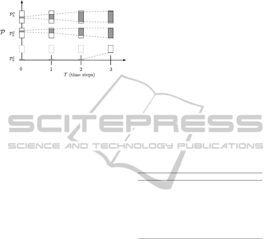
Figure 3: Temporal abstraction for a VA consisting of three

agents. White boxes indicate general bounds, grey areas

represent the boundaries at step t. Agent 1 needs two time

steps to start up and is then available at its minimum output.

functions, consider a ﬁxed rate of change constraint

c: c

min

(Σ

) := P

−P

and c

max

(Σ

) := P

. We

assume that constraints regarding minimal and max-

imal productions given in L

are also represented by

functions c

min

and c

max

(with, e.g., c

max

being a con-

stant returning P

max

or valid transitions for “jumping”

from one interval to another).

Temporal abstraction thus adds constraints ex-

cluding infeasible regions for speciﬁc time steps.

These constraints are as well only concerned with

and therefore seamlessly integrate with the AAM

found by general abstraction but further reduce the ab-

stracted search space.

∀t ∈ T : ∃[x,y] ∈ L

: x ≤ P

≤ y

In addition to the general boundaries L

that hold for

all time steps we constrain P

(the production in the

ﬁrst time step) to lie in an interval speciﬁed by L

Since these temporal boundaries converge to the gen-

eral boundaries for future time steps, it would sufﬁce

to only use them as they constitute a subset of L

. In

practice, however, it is more convenient to specify L

constraints for all time steps and use the subset of all

that actually restricts the search space and stop the

calculation after the general boundaries are reached.

5.3 Sampling Abstraction

In addition to existing abstraction mechanisms that

yield constraints shrinking the search space of the

production of a virtual agent, we are interested in

functional relationships between variables of the re-

gional model. In particular, the maximal production

change from one time step to another given the cur-

rent aggregated production is of interest to improve

the accuracy of the AAM. Even though temporal ab-

straction excludes ranges after t steps, it does not offer

any boundaries between two consecutive time steps.

A schedule that switches from minimal to maximal

production values within the limitations of L

would

be valid according to temporal abstraction but inaccu-

rate given the underlying physical systems’ possible

inertia. Similarly, a cost function could map the ag-

gregated production to the minimally required cost for

a different optimization objective.

Therefore, we acquire an abstract representation

of these functional relationships by sampling, i.e.,

solving several optimization problems and collecting

output values. Concretely, these problems consist of

the constraints in the SRM (the union of all agent

models) and introduce an additional constraint that

ﬁxes the input variable to some particular value. Us-

ing this model, the output variable is minimised or

maximised. P

(with P

still being the sum of all P

)

is, e.g., bound to be 400 and the objective is to max-

imise P

. This procedure is iterated for all future time

steps. Then, the resulting pairs of ﬁxed input and out-

put for individual time steps can be represented by a

suitable approximation method. We currently employ

piecewise linear functions that are readily supported

by MIP or constraint solvers and have been applied in

model abstraction in simulation engineering (Frantz,

1995).

Algorithm 2: Sampling Abstraction for change speeds.

Require: hX ,D,Ci is the SRM of v

Ensure: P

are pairs of the positive change speed

1: I ← s sampling points ∈ [P

min

max

]

2: procedure SAMPLING-ABSTRACTION(v, s)

3: for all {i ∈ I } do

4: C

← C ∪{(P

= i)}

5: o ← solve hX ,D, C

i : maximise P

6: P

← δ

∪ {(i,o)}

7: return pwLinear(P

)

After ﬁnding the feasible production ranges of a

VA by general abstraction as input space, we can per-

form sampling abstraction by using a number of sam-

pling points distributed across the production range

and collect the respective outputs. As of now, the

sampling points are selected equidistantly across the

full range. We sketch the approach in Algorithm 2 for

the positive production change speed P

(the nega-

tive case works analogously). As the resulting prob-

lems can still be NP-hard, we need to make sure that

the time spent for optimizing is bounded, e.g., by set-

ting a time limit and giving up on an input point if

no solution is found after that timeout is exceeded or

using an anytime algorithm that runs for a ﬁxed dura-

tion. If further properties of the function are known

such as monotonicity (x ≤ y → f (x) ≤ f (y)) or exten-

sivity (x ≤ f (x)) this information can help to shrink

the search space for the resulting sampling problems.

ICAART2014-InternationalConferenceonAgentsandArtificialIntelligence

In our evaluation case study (see Table 2) more sam-

pling points lead to increased accuracy in abstrac-

tion. In practice, an incremental approach that re-

calculates these functions in a background process is

useful to obtain more accurate representations while

initially offering a cruder variation faster. The “sam-

pled” piecewise linear function can then be used for

additional constraints in the AAM in analogy to the

optimization problem in Section 2:

∀t ∈ T \ {max T } : P

t+1

≤ P

)

∀t ∈ T \ {max T } : P

t+1

≥ P

v−

)

6 EVALUATION

The presented concept illustrated how model synthe-

sis and abstraction can be applied to hierarchical re-

source allocation problems to enable an agent-based

solution. In order to obtain a quantiﬁcation of the

speed and quality impact of this scheme, an evalua-

tion was performed for the energy management exam-

ple. A centralised solution that consists of planning

the outputs of all power plants at once is compared

to a regio-central approach using model abstraction.

This is primarily motivated by the need of comparing

optimal solutions to the ones found in a regio-central

setting.

6.1 Experimental Design

We use power plant models that are formulated as

mixed integer programs and can hence be solved

with the standard mathematical programming soft-

ware IBM ILOG CPLEX (CPLEX, 2013). Given the

same power plants and initial states, the problem is

solved with a central model and in the regio-central

approach to obtain comparable results. The following

input parameters specify an experiment run:

n the number of power plants

hc deﬁnes the strategy of hierarchy creation (we ei-

ther specify a unique maximal number of nodes

per AVPP or distinguish between leaf nodes that

only control physical power plants and inner

nodes that control other AVPPs in analogy to a B+

tree; then two parameters for AVPPs and plants

per AVPP are needed). We write h for the height

of the resulting AVPP tree.

s speciﬁes how many sampling points are used

Additionally, random seeds for all non-deterministic

aspects (combination of different constraints to plant

models, initial states and hierarchy formation) com-

plete the full speciﬁcation of one repeatable exper-

iment run. Real world data for minimal and maxi-

mal production boundaries are taken from (Deutsche

Gesellschaft f

ur Sonnenenergie e.V., 2013) and the

real world load curves are taken from (LEW Verteil-

netz GmbH, 2013). Change speeds for power plants

are generated randomly within typical boundaries. A

random hierarchy is then formed using parameter hc.

After this setup is completed, the distribution of resid-

ual load to power plants is done for 43 time steps of

15 minutes (in total a half day of prediction) with each

run assigning load for 5 time steps in advance. The

centralised model takes exactly the same form as if it

were a single AVPP responsible for all power plants.

This is to ensure that no bias is introduced by the mod-

elling or solver conﬁguration.

Several measurements are taken to compare the

quality of solutions (c, rc are subscripted for central

and regio-central, where applicable). These values are

averaged over multiple runs with differing initial ran-

dom seeds.

tr is the total runtime for the top level resource allo-

cation problem

tr/t is the runtime per time step;

abs

is the total runtime spent for abstraction; gen-

eral and sampling abstraction only have to be

performed at the beginning of the experiment

whereas temporal abstraction takes place in every

time step. We therefore divide those times into

“ﬁxed” (tr

abs

) and “variable” (tr

abs

) runtimes in

abstraction.

v is the total violation (i.e., the difference between

demand and combined production) over all con-

crete power plants to have a bottom line compari-

son relative to the demand;

ae measures the abstraction error that results if a su-

perior AVPP assigns a load to an AVPP that it

should be able to produce according to abstraction

but in fact cannot. The abstraction error is given

relative to the actually assigned load.

The experiment suite and full source code includ-

ing an instruction on how to run the experiments

used for this paper can be found online at (http://

www.informatik.uni-augsburg.de/lehrstuehle/swt/se/

staff/aschiendorfer/) in an attempt to provide repli-

cable research (Vandewalle, 2012). Each presented

experiment was run on a machine having 8 Intel

Xeon CPU 3.20 GHz cores and 14.7 GB RAM on a

64 bit Windows 7 OS with 8 GB RAM offered to the

Java 7 JVM running the abstraction algorithm as well

as the CPLEX optimiser.

SynthesisandAbstractionofConstraintModelsforHierarchicalResourceAllocationProblems

All central models used for comparison were

solved with a 30 minutes time limit per time step.

Therefore, the solver might not have produced an op-

timal solution before this time out. The time limit is

due to the 15 minute time window present in power

systems to plan ahead. As we wanted to obtain as

good a central solution as possible for comparison,

we extended this window slightly.

6.2 Experimental Results

We examine questions of interest and present the re-

sults of the experiment runs.

Scalability. Does the size of the problem impact the

performance in terms of time and quality? We expect

that after a certain number of power plants, the time

spent on abstraction is worthwhile given the runtime

performances per time step. Each hierarchy is con-

structed by taking leaf AVPPs with 20 physical power

plants each and inner nodes having a capacity of 5 (a

“B+ tree” hierarchy).

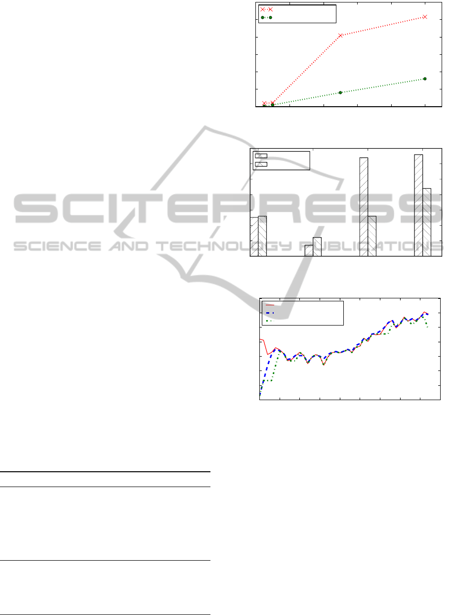
Table 1 shows how the regio-central approach

scales with rising problem size. For all input sizes,

the average violations were in similar ranges. For

n = 500 and n = 1000 the regio-central method per-

formed even better than the central model on average

as Figure 5 shows. This can occur due to the time

limit which, when exceeded, causes the states of all

power plants to remain unchanged for one time step.

Total runtimes are compared in Figure 4. In particular,

the runtimes per time step are relevant for the contin-

uous operation of the control scheme — after paying

an initial price for the construction of abstracted mod-

els, the average times are below one minute even for

Table 1: Comparison of measurements depending on differ-

ent power plant numbers. Values below the horizontal line

are only relevant to the regio-central approach. Times are

given in seconds and c and rc subscripts denote central and

regio-central, respectively.

n 50 100 500 1000

1995.29 2231.21 40850.04 51557.12

/t 46.40 51.89 950.00 1199.00

1.26% 0.36% 3.20% 3.30%

318.50 1036.22 8073.79 16018.25

/t 4.50 18.85 139.79 311.43

1.30% 0.61% 1.30% 2.20%

/tr

15.96% 46.4% 19.76% 31.07%

h 1 1 2 3

abs

125.10 224.86 2079.21 2626.7

abs

0.28 1.00 17.00 32.00

abs

/t 0.01 0.024 0.39 0.73

ae 0.01% 0.2% 0.2% 0.7%

0 200 400 600 800 1000

n (# plants)

10000

20000

30000

40000

50000

60000

t(secs)

Runtime Central

Runtime Regio-Central

Figure 4: Total runtimes central vs. regio-central.

50 100 500 1000

n (# plants)

0.0

0.5

1.0

1.5

2.0

2.5

3.0

3.5

Violation in % of target load

Central

Regio-Central

Figure 5: Violation grouped by problem size and algorithm.

0 5 10 15 20 25 30 35 40 45

t (time steps)

700000

800000

900000

1000000

1100000

1200000

1300000

1400000

P(kW h)

Residual Load

Production Regio-Central

Production Central

Figure 6: Solution for 1000 power plants and a half day in

15 minute steps, central, taken from Table 1; steps in the

central model indicate that no solution was found after 30

minutes.

1000 power plants. The percentage of runtime tr

/tr

shows that the regio-central approach needed a com-

paratively small fraction of time to come up with sim-

ilar results regarding the violation. Figure 6 visu-

alises the total violation between residual load and

production for 1000 power plants from the run shown

in Table 1. These results support the suitability of

the regio-central approach in comparison with a cen-

tral solution for practical settings in distributed energy

management.

ICAART2014-InternationalConferenceonAgentsandArtificialIntelligence

Table 2: Comparison of different sampling frequencies. As

the problem is equivalent for all runs and thus objectives are

equal for all runs, the runtimes of one central solutions are

shown here as a representative sample.

s 5 10 15 20

2235.83 2235.83 2235.83 2235.83

/t 52.00 52.00 52.00 52.00

0.36% 0.36% 0.36% 0.36%

1036.22 2104.77 2035.38 3342.05

/t 18.85 29.34 17.26 35.26

0.61% 0.49% 0.49% 0.45%

abs

224.86 842.99 1293.40 1825.62

abs

1.00 7.00 18.00 15.00

abs

/t 0.024 0.17 0.42 0.34

ae 0.2% 0.13% 0.15% 0.14%

Sampling Accuracy. How many sampling points

are needed to arrive at a good accuracy while not ex-

ceedingly spending time on abstraction? We expect

to see a tradeoff between the time spent on abstrac-

tion and the obtained accuracy. Experiments are con-

ducted for 100 power plants, half a day and varying

sampling points. Results are given in Table 2.

As we can see, the runtimes rise with the number

of sampling points due to the number of optimization

problems that have to be solved in abstraction. Com-

pared to the optimum of 0.36%, we can get as close

as to 0.45% by using 20 sampling points. However,

the runtime then even exceeds that of the central solu-

tion while providing a worse solution. A compromise

is already found at 5 sampling points which offer an

average violation of 0.61% in half of the runtime.

Hierarchy Inﬂuence. How does the hierarchy

depth affect the quality and runtime? For this exper-

iment, we compared results from 100 and 500 power

plants and varied the number of plants per AVPP. In-

teresting quantities are the abstraction error and opti-

mization objective connected to those input parame-

ters. Table 3 lists the results for different input sizes n

and plants per AVPP p. Experiments with 500 power

plants have a growing capacity towards the leaves for

performance reasons. We see that the capacity of the

AVPPs affects quality, abstraction error, and runtime

of the runs. For both 100 and 500 power plants, nodes

of 15 plants are able to obtain better solutions by hav-

ing more information available at once. Also the ab-

straction error clearly increases with smaller AVPPs

since small AVPPs imply more hierarchy levels and

thus more abstraction. Compared to Table 1 where a

hierarchy of 5 AVPPs per AVPP and 20 plants within

the leaf nodes was used, we also see that the runtimes

increase with higher capacity so a balance between

speedup by decomposition and complexity due to in-

formation collection has to be found.

Table 3: Comparison of different hierarchies. As the prob-

lem is equivalent for different AVPP capacity in the central

case, runtime of the central solution does not change for

different p.

(n/p) 100/5 100/15 500/5 500/15

2389.31 2389.31 67403.25 67403.25

/t 55.56 55.56 1567.51 1567.51

0.36% 0.36% 3.80% 3.80%

1261.49 821.00 3820.03 6832.20

/t 7.96 6.38 39.80 104.41

0.97% 0.51% 1.80% 1.62%

abs

919.28 546.75 2108.64 2342.92

abs

/t 0.005 0.007 0.008 0.057

ae 3.80% 0.3% 2.10% 0.49%

7 DISCUSSION AND

CONCLUSIONS

In this work, we presented techniques for synthesiz-

ing and abstracting constraint models that can be used

with a constraint solver in a hierarchical regio-central

fashion to reduce the complexity of a resource alloca-

tion problem. Aside from practical beneﬁts in terms

of modelling and supporting different types of agents,

we showed empirically that this approach works well

for an NP-hard problem in energy management. In

particular, the run times grow almost linearly with

the input size in the observed range of problem sizes

which is important for real-time settings while main-

taining a solution quality comparable to an optimal

solution.

However, one governing assumption states that a

formal constraint model is available for every agent

to be controlled by this scheme. In reality, this might

not always be the case — be it for practical rea-

sons, privacy issues (see e.g. Anders et al., 2013b)

or situations where a simulation is necessary to de-

termine feasibility (Bremer et al., 2010) instead of a

closed form logical formula. Therefore we plan to

integrate this approach with a learning algorithm that

constructs models of producing agents from analysing

market behaviour in a multi-agent system. Addi-

tionally, the experiments showed that the quality of

solutions and abstraction error is dominated by the

number of available sampling points. One interest-

ing direction for future work lies in investigating if

there are better choices for sampling points by draw-

ing techniques from active learning or response sur-

faces (Boyle, 2007).

Furthermore, we mainly focussed on the problem

of minimizing a deviation between demand and com-

bined production even though a more difﬁcult but eco-

SynthesisandAbstractionofConstraintModelsforHierarchicalResourceAllocationProblems

nomically important use case would optimize costs. A

two-stage optimization process that ﬁrst ﬁnds an opti-

mal solution and then tries to optimize soft constraint

violation based on constraint relationships (Schien-

dorfer et al., 2013) while staying within a predeﬁned

range around the regional optimum is planned.

ACKNOWLEDGEMENTS

The authors thank Gerrit Anders for his valuable feed-

back. This research is partly sponsored by the re-

search unit “OC-Trust” (FOR 1085) of the German

research foundation (DFG).

REFERENCES

Abouelela, M. and El-Darieby, M. (2012). Multido-

main hierarchical resource allocation for grid applica-

tions. Journal of Electrical and Computer Engineer-

ing, 2012.

Anders, G., Siefert, F., Stegh

ofer, J.-P., and Reif, W.

(2013a). Trust-based scenarios – predicting future

agent behavior in open self-organizing systems. In

Proc. of the 7th Int. Workshop on Self Organizing

Systems (IWSOS) 2013, Palma de Mallorca. Springer

Berlin Heidelberg.

Anders, G., Stegh

ofer, J.-P., Siefert, F., and Reif, W.

(2013b). A Trust- and Cooperation-Based Solution of

a Dynamic Resource Allocation Problem. In 7th IEEE

International Conference on Self-Adaptive and Self-

Organizing Systems (SASO), Philadelphia, PA. IEEE

Computer Society, Washington, D.C.

Bar-Noy, A., Bar-Yehuda, R., Freund, A., Naor, J., and

Schieber, B. (2001). A Uniﬁed Approach to Approxi-

mating Resource Allocation and Scheduling. Journal

of the ACM (JACM), 48(5):1069–1090.

Boudjadar, A., David, A., Kim, J. H., Larsen, K. G., Miku-

cionis, M., Nyman, U., and Skou, A. (2013). Hierar-

chical scheduling framework based on compositional

analysis using uppaal. In Proceedings of FACS 2013,

Lecture Notes in Computer Science. Springer.

Boyle, P. (2007). Gaussian processes for regression and op-

timisation. PhD thesis, Victoria University of Welling-

ton.

Bremer, J., Rapp, B., and Sonnenschein, M. (2010). Sup-

port vector based encoding of distributed energy re-

sources’ feasible load spaces. In Innovative Smart

Grid Technologies Conference Europe (ISGT Europe),

pages 1–8. IEEE Power Society.

Chevaleyre, Y., Dunne, P. E., Endriss, U., Lang, J.,

Lemaitre, M., Maudet, N., Padget, J., Phelps, S.,

Rodr

ıguez-Aguilar, J. A., and Sousa, P. (2006). Is-

sues in multiagent resource allocation. Informatica,

30(1):3 – 31.

Choueiry, B. Y., Faltings, B., and Noubir, G. (1994). Ab-

straction methods for resource allocation. Technical

report, Swiss Federal Institute of Technology in Lau-

sanne (EPFL).

CPLEX (2013). IBM ILOG CPLEX Optimizer. Online

Resource, last accessed December 2013: http://

www-01.ibm.com/software/commerce/optimization/

cplex-optimizer/.

Deutsche Gesellschaft f

ur Sonnenenergie e.V. (2013). En-

ergymap. Online Resource, last accessed December

2013: http://www.energymap.info/.

Frantz, F. (1995). A taxonomy of model abstraction tech-

niques. In Simulation Conference Proceedings, 1995.

Winter, pages 1413–1420.

Giunchiglia, F. and Walsh, T. (1992). A theory of abstrac-

tion. Artiﬁcial Intelligence, 57(2):323–389.

Heuck, K., Dettmann, K.-D., and Schulz, D. (2010). Elek-

trische Energieversorgung. Vieweg+Teubner. (in Ger-

man).

Hladik, P.-E., Cambazard, H., D

eplanche, A.-M., and

Jussien, N. (2008). Solving a real-time allocation

problem with constraint programming. Journal of Sys-

tems and Software, 81(1):132–149.

Kinnebrew, J. S. and Biswas, G. (2009). Efﬁcient allocation

of hierarchically-decomposable tasks in a sensor web

contract net. In Proc. of the 2009 IEEE/WIC/ACM

Int. Joint Conference on Web Intelligence and Intel-

ligent Agent Technology – Volume 02, WI-IAT ’09,

pages 225–232, Washington, DC, USA. IEEE Com-

puter Society.

Lee, K. and Fishwick, P. A. (1996). A methodology for dy-

namic model abstraction. SCS Transactions on Simu-

lation, 13(4):217–229.

LEW Verteilnetz GmbH (2013). LEW Netzdaten. On-

line Resource, last accessed December 2013: http://

www.lew-verteilnetz.de/.

Meseguer, P., Rossi, F., and Schiex, T. (2006). Soft Con-

straints. In Rossi, F., van Beek, P., and Walsh, T.,

editors, Handbook of Constraint Programming, chap-

ter 9. Elsevier.

Pelikan, M. and Goldberg, D. E. (2000). Hierarchical prob-

lem solving by the bayesian optimization algorithm.

In Proc. of the Genetic and Evolutionary Computation

Conference 2000, pages 267–274. Morgan Kaufmann.

Ramchurn, S. D., Vytelingum, P., Rogers, A., and Jennings,

N. R. (2012). Putting the ’smarts’ into the smart grid:

a grand challenge for artiﬁcial intelligence. Commun.

ACM, 55(4):86–97.

Santos, C., Zhu, X., and Crowder, H. (2002). A mathemat-

ical optimization approach for resource allocation in

large scale data centers. Technical Report HPL-2002-

64, HP Labs.

Schiendorfer, A., Stegh

ofer, J.-P., Knapp, A., Nafz, F., and

Reif, W. (2013). Constraint relationships for soft con-

straints. In Bramer, M. and Petridis, M., editors, Re-

search and Development in Intelligent Systems XXX.

Springer London.

Stegh

ofer, J.-P., Anders, G., Siefert, F., and Reif, W.

(2013a). A system of systems approach to the evo-

lutionary transformation of power management sys-

tems. In Proceedings of INFORMATIK 2013 – Work-

shop on “Smart Grids”, Lecture Notes in Informatics.

Bonner K

ollen Verlag.

ICAART2014-InternationalConferenceonAgentsandArtificialIntelligence

Stegh

ofer, J.-P., Behrmann, P., Anders, G., Siefert, F., and

Reif, W. (2013b). HiSPADA: Self-organising hierar-

chies for large-scale multi-agent systems. In Proceed-

ings of the IARIA International Conference on Auto-

nomic and Autonomous Systems (ICAS) 2013. IARIA.

Van Zandt, T. (1995). Hierarchical computation of the re-

source allocation problem. European Economic Re-

view, 39(3-4):700–708.

Vandewalle, P. (2012). Code sharing is associated with re-

search impact in image processing. Computing in Sci-

ence Engineering, 14(4):42–47.

Yokoo, M., Durfee, E. H., Ishida, T., and Kuwabara, K.

(1998). The distributed constraint satisfaction prob-

lem: Formalization and algorithms. IEEE Transac-

tions on Knowledge and Data Engineering, 10:673–

685.

SynthesisandAbstractionofConstraintModelsforHierarchicalResourceAllocationProblems