
Agent-based Manufacturing in a Production Grid
Adapting a Production Grid to the Production Paths
Leo van Moergestel
1
, Dani
¨
el Telgen
1
, Erik Puik
1
and John-Jules Meyer
2
1
Institute of ICT, HU University of Applied Sciences, Utrecht, The Netherlands
2
Information and Computing Sciences, Utrecht University, Utrecht, The Netherlands
Keywords:
Multiagent-based Manufacturing, Reconfigurable Manufacturing System.
Abstract:
In standard mass production, batch processing is widely accepted. The advantage of batch processing is that
production equipment can be placed in a so called production line. A product only has to follow this line
and all production steps will be performed. However, this set-up is not adequate for low cost small quantity
production. In this paper, agile production of small quantities in a grid of reconfigurable production machines
called equiplets is described. One of the challenges in this approach is the transport of the product between
the equiplets during production. This paper describes some heuristic methods to reduce the average path a
product has to follow in the production grid.
1 INTRODUCTION
Standard mass production is mostly batch-oriented.
This means that a kind of pipeline production model
is used. Normally this pipeline produces a huge quan-
tity of a certain product. Though this approach is very
cost-effective, it lacks flexibility and agile adaptation
as well as low-cost production of small batches.
In a global view, the production model that is pre-
sented in this paper consists of a set of manufacturing
machines. However the production is not pipeline-
based because the aim of this model is to produce
different products in parallel. Every product needs
its own, possibly unique, set of manufacturing ma-
chines. Because the production is not pipeline-based,
the transport between the manufacturing machines
becomes an important issue.
2 GRID MANUFACTURING
In grid production, manufacturing machines are
placed in a grid topology. Every manufacturing ma-
chine offers one or more production steps and by
combining a certain set of production steps, a product
can be made. This means that when a product requires
a given set of production steps and the grid has these
steps available, the product can be made. The soft-
ware infrastructure that has been used in our grid, is
agent-based. Agent technology opens the possibilities
to let this grid operate and manufacture different kinds
of products in parallel, provided that the required pro-
duction steps are available (Moergestel et al., 2011).
2.1 Manufacturing Model and Related
Work
The manufacturing machines that have been built in
our research group are cheap and versatile. These
machines are called equiplets and consist of a stan-
dardized frame and subsystem on which several dif-
ferent front-ends can be attached. The type of front-
end specifies what product steps a certain equiplet can
provide. This way every equiplet acts as a reconfig-
urable manufacturing system (RMS).The equiplet is
in software represented by a so called equiplet agent.
This agent advertises its production steps to a black-
board that is available in a multi agent system where
also so-called product agents live. A product agent is
responsible for the manufacturing of a single product
and knows what to do, the equiplet agents knows how
to do it.
In (Koren et al., 1999) the concepts of reconfigurable
manufacturing systems are introduced and explained.
A more recent article about this subject can be found
in (Bensmaine et al., 2013). In this work, to take
full advantage of the reconfigurability of RMSs, a
new approach is proposed using genetic algorithms
and a simulation based optimization for process plan-
ning for a single product type. The proposed approach
342
van Moergestel L., Telgen D., Puik E. and Meyer J..
Agent-based Manufacturing in a Production Grid - Adapting a Production Grid to the Production Paths.
DOI: 10.5220/0004758803420349
In Proceedings of the 6th International Conference on Agents and Artificial Intelligence (ICAART-2014), pages 342-349
ISBN: 978-989-758-015-4
Copyright
c
2014 SCITEPRESS (Science and Technology Publications, Lda.)

copes with market uncertainty and demands fluctua-
tion in order to satisfy demands within their deadlines
and with a minimum total cost. Our work is agent-
based and is not limited to a single product type.
The concept of grid production in a grid of
equiplets is introduced in (anon.ref.) Using agent
technology in industrial production is not new though
still not widely accepted. Important work in this field
has already been done. Paolucci and Sacile(Paolucci
and Sacile, 2005) give an extensive overview of what
has been done in this field. Their work focuses on
simulation as well as production scheduling and con-
trol.The main purpose to use agents in (Paolucci and
Sacile, 2005) is agile production and making complex
production tasks possible by using a multi-agent sys-
tem. Agents are also introduced to deliver a flexible
and scalable alternative for a manufacturing execu-
tion system (MES) for small production companies.
The roles of the agents in this overview are quite di-
verse. In simulations agents play the role of active en-
tities in the production. In production scheduling and
control, agents support or replace human operators.
Agent technology is used in parts or subsystems of
the manufacturing process. We on the contrary based
the manufacturing process as a whole on agent tech-
nology. In our case a co-design of hardware and soft-
ware was the basis.
Bussmann and Jennings (Bussmann et al.,
2004)used an approach that compares to our ap-
proach. The system they describe introduced three
types of agents, a workpiece agent, a machine agent
and a switch agent. Some characteristics of their so-
lutions are:
• The production system is a production line that is
built for a certain product. This design is based on
redundant production machinery and focuses on
production availability and a minimum of down-
time in the production process. Our system is
a grid and is capable to produce many different
products in parallel;
• They use a special infrastructure for the logistic
subsystem, controlled by so called switch agents.
The logistic subsystem consists of two transport
belts running in opposite direction. The switch
agent can move a product from one transport belt
to another, creating loops and the possibility to
visit a previous production machine. In our sit-
uation, cheap mobile robot platforms will be used
to transport the product including its parts form
equiplet to equiplet. The product agent has the re-
sponsibility for this transport in its role of guiding
the product.
There are however important differences to our ap-
proach. The solution presented by Bussmann and Jen-
nings has the characteristics of a production pipeline
and is very useful as such, however it is not meant to
be an agile multi-parallel production system as pre-
sented here. The work of Xiang and Lee (Xiang and
Lee, 2008) presents a scheduling multiagent-based
solution using swarm intelligence. This work uses ne-
gotiating between job-agents and machine-agents for
equal distribution of tasks among machines. In our
system there is no need for balancing the load be-
tween equiplets, because these production platforms
are cheap and their use depends on what kind of pro-
duction steps are needed at a certain moment.The
work of (Minguez et al., 2010) is based on service
oriented architecture (SOA) instead of agents technol-
ogy as presented in the current paper to achieve an
agile and fast responding production. Their focus is
also not on co-design, but on improvement of existing
production systems.
2.2 Agents-based Production
As mentioned in section 2.1, production control is
agent-based (Moergestel et al., 2011). The equiplet
is controlled by an equiplet agent. This agent is re-
sponsible for a certain equiplet and its front-end. It
interacts with the production hardware, other agents
in the grid and possibly, in a semi-automated environ-
ment, with a human equiplet operator. An equiplet
agent will:
• announce its steps in its role of publisher on a
blackboard that is readable for all product agents;
• in its role of waiter, wait for clients (product
agents) to arrive;
• in its role of step performer, perform production
steps and inform clients about results of a step.
In all its roles it will also inform product agents about
the feasibility of steps in combination with certain pa-
rameters.
The product agent has three roles:
1. planning: in this role the agent selects the appro-
priate set of equiplets. It first asks the equiplets of-
fering a certain production step, if this step is fea-
sible for a given set of parameters and how long
the step will take on that specific equiplet. It also
tries to bundle steps in a sequence that are per-
formed by the same equiplet (Moergestel et al.,
2011). The next phase in the planning is calculat-
ing the path within the grid. When all planning is
done the agent can start with the next role;
2. scheduling: in this role the agent tries to schedule
the production steps on the given equiplets, taken
into account the travel time between the equiplets
and the estimated production time per step;
Agent-basedManufacturinginaProductionGrid-AdaptingaProductionGridtotheProductionPaths
343

3. guiding: in this role the product agent guides the
product to be made along the equiplets and col-
lects manufacturing data to be kept in a produc-
tion log for that specific product. In this role the
recovery from errors and if required, rescheduling
is done.
The scheduling is implemented as an atomic action
for the product agent. The product agent will sched-
ule all production steps it needs, while other agents
are temporarily blocked from scheduling. This will
prevent deadlocks. The products allocates available
free timeslots for all equiplets it needs for produc-
tion. If the complete path of steps is within the dead-
line, the scheduling is considered successful. If the
scheduling fails the product agent will do a resched-
ule. This reschedule is based on the ”earliest dead-
line first” (EDF) approach. This approach turned out
to give a high success rate (Moergestel et al., 2012).
The product agent that encounters a failing schedul-
ing, will ask all agents with a later deadline to hand
over their scheduling and the product agent with the
failing scheduling will try to reschedule itself and all
agents having a later deadline according to the EDF-
approach. If this results in a feasible scheduling for
all involved product agents, the new scheduling will
be reported to all agents that temporally gave up their
scheduling. If this rescheduling fails for one or more
agents, the product agent that did the rescheduling
will report a scheduling failure to its maker and gives
up. The other agents continue with their old schedul-
ing schemes.
Summarized: each equiplet offers a set of produc-
tion step S
Eq
i
= {σ
a
, σ
b
, ˙...}. A grid with N equiplets
offers a set S
grid
that is the union of all sets offered
by the equiplets: S
grid
=
S
N
i=1
S
Eq
i
Every product
needs in its simplest form a tuple of production steps
< σ
i
, σ
j
, ˙... >. The product agent tries to find a match
for its steps within the grid. More complex products
can be considered as the result of a set or tuple of tu-
ples of production steps.
When all product agents have arranged their plan-
ning and scheduling, every path the product has to fol-
low during its production is a kind of a random walk
within the grid. Because the equiplets are reconfig-
urable machines it is a good idea to adapt the posi-
tion of equiplets in the grid to the set of products to
be manufactured. This should result in an optimisa-
tion of the average production path for the individual
products to be made.
2.3 Similarities and Differences between
Batch and Grid Production
Both batch and grid production are based on the con-
cept of a production step. In a batch environment
these steps have the same sequence for all products.
Also in batch production the duration of steps is nor-
mally the same, so a pipeline of a chain of production
steps is easy to implement and effective. The draw-
back is that all products should be similar to make
this concept work. In grid production the duration
of steps can vary without disturbing the production.
Also the sequence of steps can vary among products
opening the possibility to produce several different
products in parallel. The drawback here is the com-
plication of different paths along the production ma-
chines. Instead of a transport belt or a similar solu-
tion, a much more complicated transport system is re-
quired (Bussmann et al., 2004). The transport system
can be optimised if the position of the production ma-
chines within the grid is adapted to the set of paths
that are required for production. This is the subject of
the research described in this paper. The equiplets are
reconfigurable machines. The product agents make
their planning according to the capabilities offered by
the equiplets. Combining this information the ques-
tion arises: is it possible to adapt the positions of the
equiplets in the grid, so that the average length of the
paths of the products is shorter than in case of a ran-
dom walk within the grid? The length of the path
in the grid is also referred to as the amount of hops,
where a hop is a path between two adjacent nodes. In
our model the length of a path between two adjacent
nodes is 1.
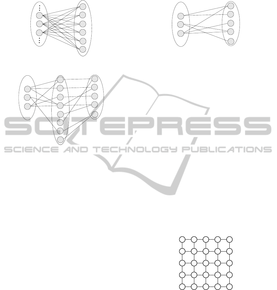
To explain in a more formal way the differences
between batch production and grid production, con-
sider a batch production system. This system can be
represented by a tripartite graph as depicted in fig-
ure 1. Every step (member of set S) matches one sin-
gle production machine (member of set E). All prod-
ucts (P) use all available steps in a sequence, one by
one. This tripartite graph can be transformed to the
bipartite graph of figure 4, where only products (P)
and production machines (E) are involved. The pro-
P S E
Figure 1: A batch process as a matching tripartite graph.
ICAART2014-InternationalConferenceonAgentsandArtificialIntelligence
344
P
E
Figure 2: A batch process as a matching tripartite graph.
P S
E
Figure 3: Grid-based manufacturing system.
duction in a grid can be represented by the tripartite
graph of figure 3. Here it can be seen that not all prod-
ucts use all the available steps and some production
machines (Equiplets, denoted by E) offer more than a
single production step. After the planning phase, the
product agents have chosen their set of equiplets and
the tripartite graph can be transformed to the bipartite
graph of figure 4. This bipartite graph is in this case
the result of a certain planning. If a step is offered by
two or more equiplets and a product agent selects a
different equiplet to perform a step, the resulting bi-
partite graph is also different. In case of batch-based
production, there are no choices of this kind. Apart
from the fact that this bipartite is not necessarily a
complete graph (where every node from set P matches
with all nodes from set E), there is another important
difference. The edges of the graph are not used in a
fixed sequence (in figure 2 from top to bottom for ev-
ery product), but the time they are active should be
scheduled among all other edges involved. This plan-
ning and scheduling is described in (Moergestel et al.,
2012).
3 ADAPTION OF THE GRID
There are several ways to adapt the grid to the pro-
duction paths. Two possibilities used in this research
are:
P
E
Figure 4: Grid-based manufacturing system.
1. the grid can be configured or reconfigured accord-
ing to information about the load or usage of the
equiplets;
2. a configuration can be calculated according to the
amount of inter-equiplet hops used by the produc-
tion paths.
For both approaches an alternative brute force method
could be used. For a reasonable sized grid (e.g. 4 ×4
or bigger) this requires a huge amount of calculation
because of the fast increasing set of possible configu-
rations being in the order of (N ×N)! for an N ×N-
grid. A better solution would be a heuristic approach
that might lead to an acceptable result. To get a feel-
ing about what heuristic might be a good approach,
this research used two possibilities as already men-
tioned before.
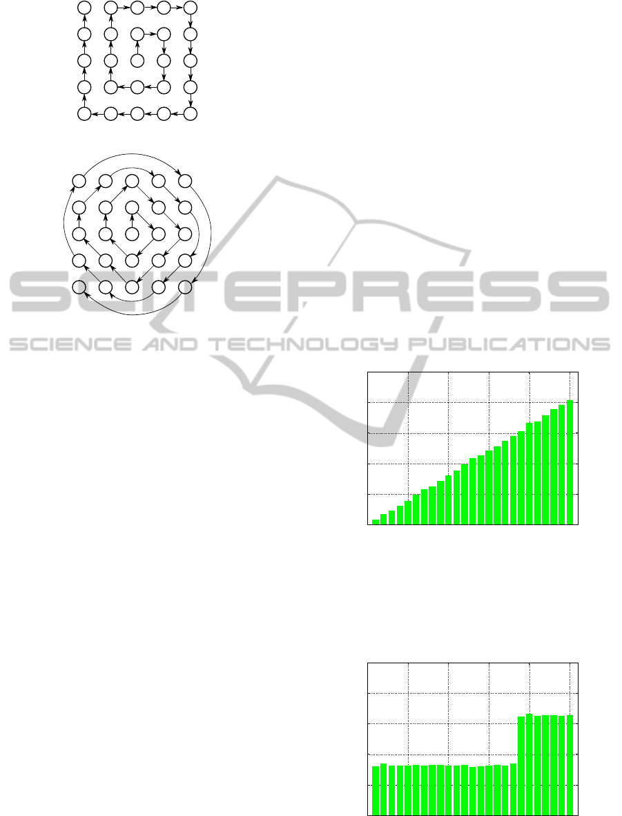
The basic idea is based on the fact that nodes in a
grid have different average values for reaching other
nodes in the grid. For a 5 ×5-grid these values are
shown in figure 5. This means that from a corner
point, the average path to any other node in the grid
is 4, while the node in the center has an average path
of 2.4 to any other node. This means that it is wise to
4
3.4
3.2
2.8
2.6
2.4
3.4
3.4
3.4 3.4
3.4
3.4
2.6 2.6
2.6
3.2
2.8 2.8
2.8
3.2
3.4
4
44 3.2
Figure 5: Reachability of nodes in the grid.
place the most heavily used equiplet at the center and
then grouping other heavily used equiplets around it.
For this grouping two patterns have been used. The
first pattern, grid pattern 1, is shown in figure 6. Here
we start at the hot-spot in the middle of the grid and
construct a path among other nodes also having a low
value for the average path, but we construct a path that
has only one hop between two consecutive nodes. In
figure 7 an alternative path, grid pattern 2, is shown.
This path follows the lists of shortest average paths
that can be derived from figure 5. We expect both
Agent-basedManufacturinginaProductionGrid-AdaptingaProductionGridtotheProductionPaths
345
4
3
2
2
1
0
3
3
3 3
3
3
1 1
1
2
2 2
2
2
3
4
44 2
Figure 6: A path along the nodes.
4
3
2
2
1
0
3
3
3 3
3
3
1 1
1
2
2 2
2
2
3
4
44 2
Figure 7: An alternative path along the nodes.
patterns to give an improvement under certain circum-
stances. Pattern 2 because of the fact that heavily used
equiplets are placed at easily reachable positions from
any point in the grid. Pattern 1 looks similar, but has
the order of its sequence separated by only one hop.
To test our approach, several scenarios are gener-
ated using a Monte Carlo method. We generated sets
of production steps needed for a product and mapped
these to the available equiplets. A set containing
many different products was thus generated. From
these artificially generated production sets a matrix
(1) is constructed that has all the transitions between
all pairs of equiplets. This matrix of transitions con-
sists of elements α
i j
having the number of transitions
from equiplet i to equiplet j while α
ji
shows the num-
ber of transitions from equiplet j to equiplet i.
α
11
α
12
. . . α
1n
α
21
a
22
. . . α
2n
.
.
.
.
.
.
.
.
.
.
.
.
α
n1
α
n2
. . . α
nn
(1)
For computing purposes another matrix was also con-
structed using the values of matrix 1. In this matrix we
only look at the transition between equiplets neglect-
ing the direction of the transitions. This matrix is not
an optimisation, but a different representation. This
results is a matrix (2) having only non-zero values in
the lower left triangle below the diagonal. Where the
non-zero values β
i j
= α
i j
+ α
ji
: ∀j < i. In the next
sections this type of matrix is referred to as a triangle
matrix. In one of the computations in section 4 this
triangle matrix is the starting point.
0 0 . . . 0
β
21
0 . . . 0
.
.
.
.
.
.
.
.
.
.
.
.
β
n1
βn2 . . . 0
(2)
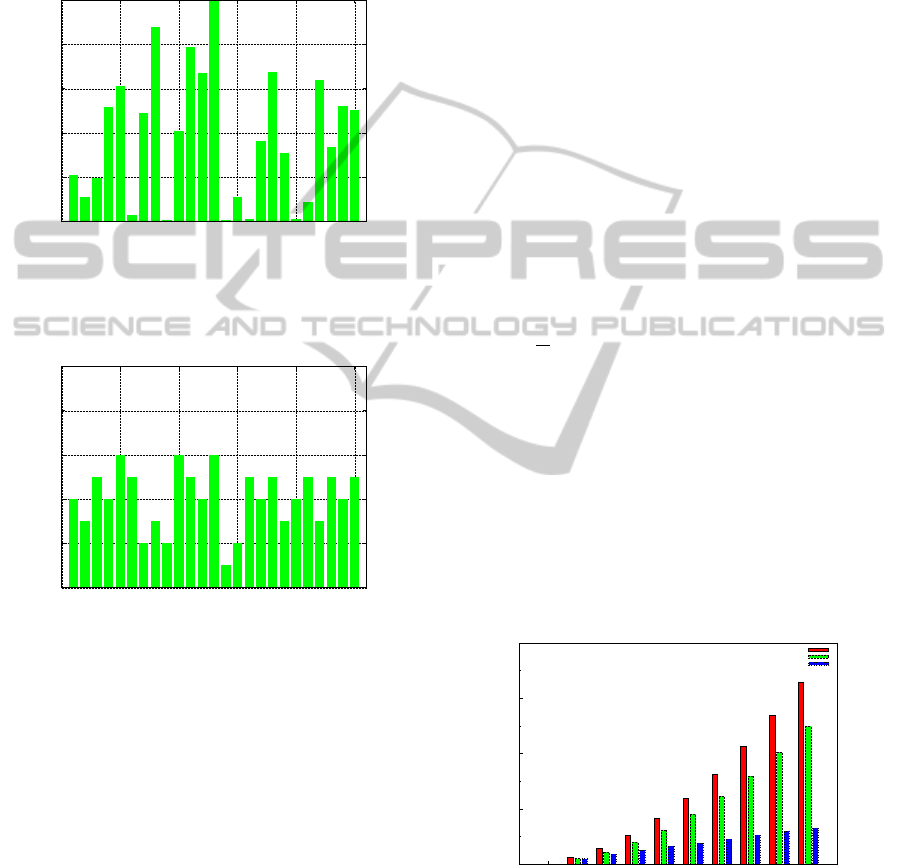
3.1 Scenarios
To test the adaption software, several scenarios were
generated. All scenarios are based on 10000 products
that could use 25 equiplets in a 5 ×5 configuration.
Following is a description of the scenarios:
A All products paths are randomly generated with-
out making some equiplets special. The usage is
almost equally distributed over all equiplets.
B Again a randomly generated set of product paths,
but now there is a linear increase of usage among
the equiplets, making equiplet 25 much more pop-
ular than equiplet 1. Figure 8 shows the distribu-
tion of the equiplet usage. The equiplets are num-
bered from 1 to 25.
0
2000
4000
6000
8000
10000
0 5 10 15 20 25
Usage
Equiplet
Figure 8: Equiplet usage distribution for scenario B.
C In this set of product paths 25% of the equiplets
are used twice as much. This might be the case
if equiplets offer more than one production step.
(see figure 9).
0
2000
4000
6000
8000
10000
0 5 10 15 20 25
Usage
Equiplet
Figure 9: Equiplet usage distribution for scenario C.
ICAART2014-InternationalConferenceonAgentsandArtificialIntelligence
346
D A test set that is purely batch-based. 10000 prod-
ucts using all the 25 equiplets equally in a batch
production situation.
E A test set having several different products with
comparable paths, but not of the same length (see
figure 10).
0
2000
4000
6000
8000
10000
0 5 10 15 20 25
Usage
Equiplet
Figure 10: Equiplet usage distribution for scenario E.
F A testset 10 different products, resulting in 10 sets
of 1000 products. (see figure 11).
0
2000
4000
6000
8000
10000
0 5 10 15 20 25
Usage
Equiplet
Figure 11: Equiplet usage distribution for scenario F.
4 COMPUTATIONS
The first approach only looks at the usage of the
equiplets and puts the most popular equiplet at the
hot spot. The stepwise description of the computation
looks like:
matrix = ConstructMatrixOfTransitions(input);
tr_matrix = TransformToTriangle(matrix);
list = CalculateUsageOfEquiplet(tr_matrix);
// Make a list of usage and equiplet-number
SortList(list; // sort this list according
// to usage, putting the highest on top
grid = GenGrid(list, gridpattern); //Generate
// a grid using list and pattern (1 or 2)
CalculatePathLength(grid); //Use this grid to
// calculate the actual average pathlength
If the transitions are taken into account, the situation
is a litle bit more complicated.
matrix = ConstructMatrixOfTransitions(input);
list = MakelistOfTriplets(matrix); //Make
// list of triplets of all transitions:
// #num eq-src eq-dst
list = SortList(list); //sort list to #num
equipList = CreateListOfEquiplets(list){
//starting at the top and from there
// following eq-dst as the next eq-src
IF(loop) Find_Next_Unused_triplet(list);
}
grid = GenGrid(equipList, gridpattern);
//Generate a grid using list and pattern
CalculatePathLength(grid); //Use this grid to
// calculate the actual average pathlength
4.1 Grid versus Line and Circle
Before discussing the results of the computations de-
scribed in de previous subsection, we first made some
calculations on the average number of hops for a ran-
dom path between nodes on a line, on a circle and
in a grid. In figure 12 the number of hops is plotted
against
√
N, where N is the number of nodes among
the line, the circle or in the grid. The increase of the
average path length (number of hops) is the highest
for nodes put on a line. So a random walk along a
line is behaving bad, when the number of nodes in-
creases. When the nodes are placed on a circle, there
is some improvement because of the effect that the
largest distance now is over only halfway around the
circle. When the same calculation is done for the grid,
a slow and almost linear increase will be the result as
shown in figure 12. Thus from these three possibili-
ties, the grid is by far the best choice.
0
10
20
30
40
1 2 3 4 5 6 7 8 9 10
Average number of hops
SQRT(N)
line
circle
grid
Figure 12: Number of hops for different configurations of
N nodes.
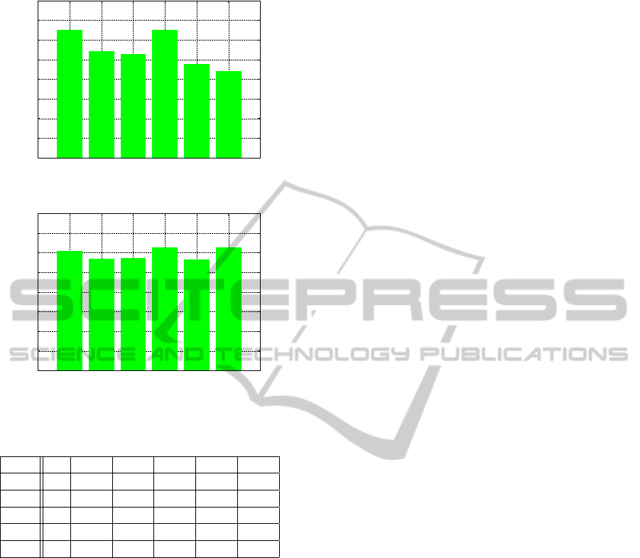
4.2 Results
The results of the calculations are plotted as his-
tograms. Every histogram shows the results for one
Agent-basedManufacturinginaProductionGrid-AdaptingaProductionGridtotheProductionPaths
347
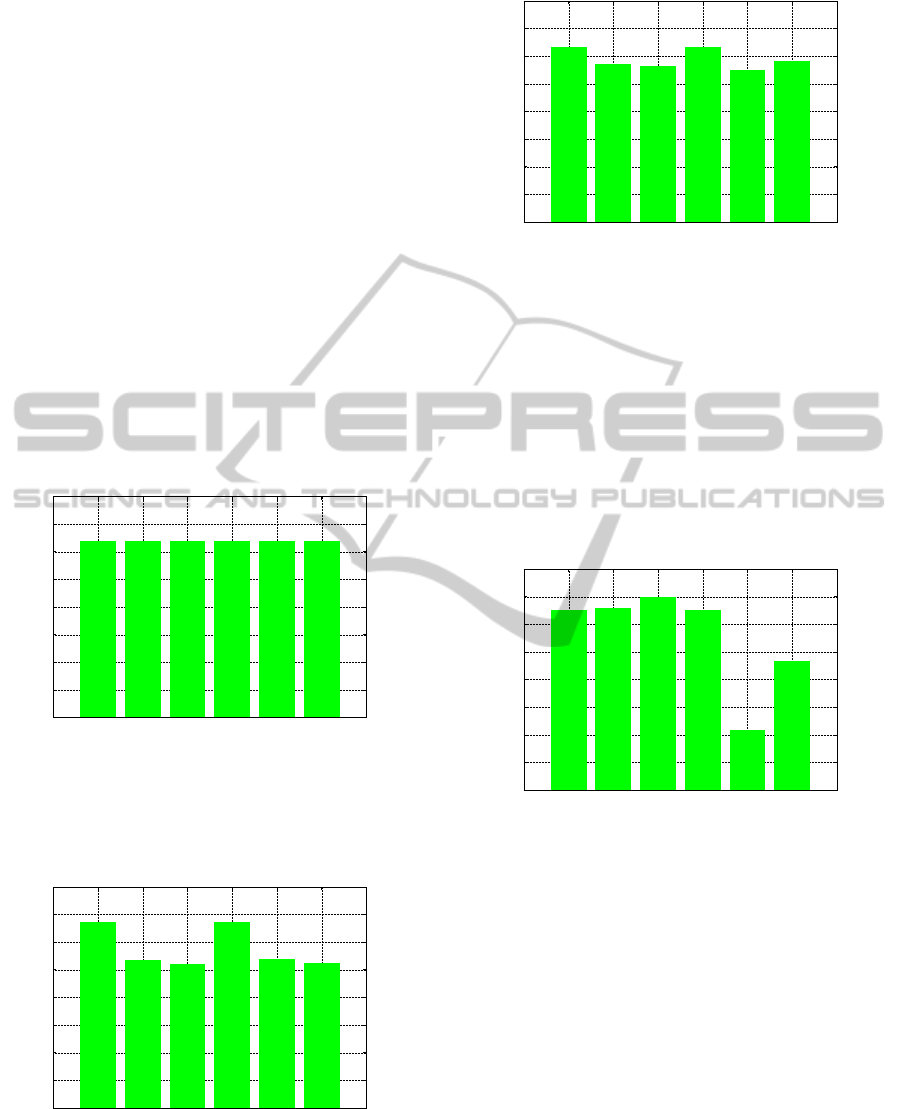
scenario. The numbered bars represent the fol-
lowing tests:
1. random grid configuration, used as a reference
measurement;
2. using grid pattern 1 from figure 6 with equiplets
ordered according to usage;
3. using gridpattern 2 from figure 7 with equiplets
ordered according to usage;
4. again a random grid configuration (different from
1);
5. using gridpattern 1 from figure 6 with equiplets
ordered according to transition frequency;
6. using gridpattern 2 from figure 7 with equiplets
ordered according to transition frequency;
Figure 13 shows the results for the purely random sit-
uation. In this case no gain is possible, because all
equiplets have almost the same load and all transis-
tions have the same probability. Figure 14 shows the
0
0.5
1
1.5
2
2.5
3
3.5
4
0 1 2 3 4 5 6 7
Average Path
Test number
Figure 13: Scenario A with random use of equiplets.
results for scenario B. Here we see a decrease of the
average path length. There is not much difference be-
tween the different approaches. In figure 15 the re-
0
0.5
1
1.5
2
2.5
3
3.5
4
0 1 2 3 4 5 6 7
Average Path
Test Number
Figure 14: Scenario B with increasing use of equiplets.
sults are shown for scenario C. Again a decrease of
average path length. The best result is test number
5 where grid pattern 1 is used in combination with
0
0.5
1
1.5
2
2.5
3
3.5
4
0 1 2 3 4 5 6 7
Average Path
Test Number
Figure 15: Scenario C with two overlapping sets of
equiplets.
the number of inter-equiplet hops. The results of a
pure batch scenario is shown in figure 16. Normally
in a batch the production machines are in-line sepa-
rated by one single hop. This possibility is discovered
by test 5, using grid pattern 1 in combination with
the number of inter-equiplet hops. When we look at
the results based on the usage of equiplets, there is
no gain at all. This has to do with the fact that all
equiplets are equally used, so sorting does not make
any difference. In figure 17 the results for scenario E
0
0.5
1
1.5
2
2.5
3
3.5
4
0 1 2 3 4 5 6 7
Average Path
Test Number
Figure 16: Scenario D with a single batch.
are shown. Here we also see a gain and in this case
test 6, using grid pattern 2 in combination the number
of inter-equiplet hops is the best solution. The final
histogram of figure 18 shown the results for test 10.
Here the gain is minimal but still available in three of
the experiments.
5 DISCUSSION AND FUTURE
WORK
In table 1, the percentage of reduction in hops is cal-
culated for all scenarios and heuristics by taking the
average of 3.2 and comparing it with the actual results
shown in the graphs of the previous section. The high-
est profit is printed in bold typeface. It turns out that
ICAART2014-InternationalConferenceonAgentsandArtificialIntelligence
348
0
0.5
1
1.5
2
2.5
3
3.5
4
0 1 2 3 4 5 6 7
Average Path
Test Number
Figure 17: Scenario E with repeated tuples of equiplets.
0
0.5
1
1.5
2
2.5
3
3.5
4
0 1 2 3 4 5 6 7
Average Path
Test Number
Figure 18: Scenario with 10 different batches of similar
products.
Table 1: Reduction of hops in %.
Test A B C D E F
1, 4 0 0 0 0 0 0
2 0 16.3 10.9 -3 15.6 10.9
3 0 18.5 12 -9 17.8 10.6
5 0 16.3 14.4 66.3 25.6 11.6
6 0 18.4 9.4 28.2 31.2 2
test 5 gives the best results, but not for all scenarios,
having test 3 as a winner for scenario B and test 6 for
scenario E. The approach presented here can be inte-
grated with the grid software architecture (Moergestel
et al., 2013). In the architecture, provisions have been
made to implement a monitoring system. This system
can produce the usage of the equiplets and the inter-
equiplet transport in the past and also by looking at
the planning blackboard the use and transport in the
near future. This information can be used for opti-
mising the grid. This way the grid control software
can adapt to the production situation. In future re-
search other grid patterns should be investigated and
specially the scenarios in a real agile production envi-
ronment should be studied to get an understanding of
what might be adequate grid scenarios.
6 CONCLUSIONS
The amount of transportation can be reduced by
heuristic methods. The actual profit depends on the
set of products to be made. The best solution seems
to be to use different methods to find a solution and fi-
nally implement the best solution. By automating this
approach the grid will adapt itself to changing pro-
duction requirements. So far only a small production
grid has been implemented, but when bigger grids are
built within the future, the tools to let it adapt are
ready for use. It would be interesting to see if real-
world problems are akin to the situations that have
been presented in this paper. Our expectation is that
sets of pure random sequences that cannot be opti-
mized by the methods presented here, might be ex-
ceptional cases, because of the fact that certain prod-
uct steps are related and mostly used in a sequence,
some steps are used at the beginning and other steps
mostly at the end of production.
REFERENCES
Bensmaine, A., Dahane, M., and Benyoucef, L. (2013). A
simulation-based genetic algorithm approach for pro-
cess plans selection in uncertain reconfigurable envi-
ronment. IFAC Conference on Manufacturing Mod-
elling, Management and Control, pages 2002–2007.
Bussmann, S., Jennings, N., and Wooldridge, M.
(2004). Multiagent Systems for Manufacturing Con-
trol. Springer-Verlag, Berlin Heidelberg.
Koren, Y., Jovane, F., Heisel, U., Moriwaki, T., G., P., G.,
U., and H., V. (1999). Reconfigurable manufacturing
systems. Keynote paper. CIRP Annals, 48(2):6–12.
Minguez, J., Lucke, D., Jakob, M., Constantinescu, C., and
Mitschang, B. (2010). Introducing soa into production
environments - the manufacturing service bus. Pro-
ceedings of the 43rd. CIRP International Conference
on Manufacturing Systems, pages 1117–1124.
Moergestel, L. v., Meyer, J.-J., Puik, E., and Telgen,
D. (2011). Decentralized autonomous-agent-based
infrastructure for agile multiparallel manufacturing.
ISADS 2011 proceedings, pages 281–288.
Moergestel, L. v., Meyer, J.-J., Puik, E., and Telgen, D.
(2012). Production scheduling in an agile agent-based
production grid. IAT proceedings, pages 293–298.
Moergestel, L. v., Meyer, J.-J., Puik, E., and Telgen, D.
(2013). A versatile agile agent-based infrastructure
for hybrid production environments. IFAC Manufac-
turing Modelling, Management, and Control (MIM)
2013 proceedings, 7:210–215.
Paolucci, M. and Sacile, R. (2005). Agent-based manufac-
turing and control systems : new agile manufacturing
solutions for achieving peak performance. CRC Press,
Boca Raton, Fla.
Xiang, W. and Lee, H. (2008). Ant colony intelligence
in multi-agent dynamic manafacturing scheduling.
Engineering Applications of Artificial Intelligence,
16(4):335–348.
Agent-basedManufacturinginaProductionGrid-AdaptingaProductionGridtotheProductionPaths
349
