
Measuring Cluster Similarity by the Travel Time
between Data Points
Yonggang Lu
1
, Xiaoli Hou
1
and Xurong Chen
2,3
1
School of Information Science and Engineering, Lanzhou University, Lanzhou, Gansu 730000, China
2
Institute of Modern Physics, Chinese Academy of Sciences, Lanzhou, Gansu 730000, China
3
Institute of Modern Physics of CAS and Lanzhou University, Lanzhou, Gansu 730000, China
Keywords: Clustering, Travel Time, Hierarchical Clustering, Similarity Measure.
Abstract: A new similarity measure for hierarchical clustering is proposed. The idea is to treat all the data points as
mass points under a hypothetical gravitational force field, and derive the hierarchical clustering results by
estimating the travel time between data points. The shorter the time needed to travel from one point to
another, the more similar the two data points are. In order to avoid the complexity in the simulation using
molecular dynamics, the potential field produced by all the data points is computed. Then the travel time
between a pair of data points is estimated using the potential field. In our method, the travel time is used to
construct a new similarity measure, and an edge-weighted tree of all the data points is built to improve the
efficiency of the hierarchical clustering. The proposed method called Travel-Time based Hierarchical
Clustering (TTHC) is evaluated by comparing with four other hierarchical clustering methods. Two real
datasets and two synthetic dataset families composed of 200 randomly produced datasets are used in our
Experiments. It is shown that the TTHC method can produce very competitive results, and using the
estimated travel time instead of the distance between data points is capable of improving the robustness and
the quality of clustering.
1 INTRODUCTION
Clustering is an important unsupervised data
analysis tool to explore data structures. It has been
applied to a variety of applications, such as pattern
classification, data mining, image processing and
machine learning (Omran et al., 2007; Filippone et
al., 2008; Jain, 2010). Based on the structure of the
results, the clustering methods can be divided into
two different groups: partitional and hierarchical.
Partitional clustering method produces a single
partition, while hierarchical clustering method
produces a rooted tree of data points, called a
dendrogram, from which different and consistent
partitions can be derived at different levels (Omran
et al., 2007; Filippone et al., 2008; Jain, 2010).
These partitions are consistent in a sense that they
form a total order set if the refinement relation is
considered. Because the result of hierarchical
clustering can be used to analyze the structure of the
data at different levels, it has been widely used in
different areas, such as document clustering (Gil-
García et al., 2010), the analysis of gene expression
data, regulatory networks and protein interaction
networks (Assent, 2012; Yu et al., 2006; Wang et
al., 2011). There are usually two different
approaches for hierarchical clustering:
agglomerative and divisive. The agglomerative
method follows a bottom-up approach: initially each
data point is in a different cluster, and then the two
most similar clusters are merged at each step until a
single cluster is produced. The divisive method
follows a top-down approach: initially all the data
points are in a single cluster and the selected cluster
at each step is divided into two clusters until no
more division can be made. Four commonly used
agglomerative methods are: Single Linkage,
Complete Linkage, Average Linkage and Ward’s
method (Omran et al., 2007; Murtagh et al., 2012).
Although there are lots of progresses made recently,
challenges remain on how to improve the efficiency
and the quality of hierarchical clustering methods to
address many important problems (Murtagh et al.,
2012).
Gravitational clustering (Wright, 1977) is an
interesting and effective method which performs
clustering by simulating natural processes. All the
14
Lu Y., Hou X. and Chen X..
Measuring Cluster Similarity by the Travel Time between Data Points.
DOI: 10.5220/0004761800140020
In Proceedings of the 3rd International Conference on Pattern Recognition Applications and Methods (ICPRAM-2014), pages 14-20
ISBN: 978-989-758-018-5
Copyright
c
2014 SCITEPRESS (Science and Technology Publications, Lda.)

data points are considered to be mass points which
can move under interactions following the Newton’s
Law of gravitation. Then the data points which move
close to each other are grouped to a same cluster.
This way, the clusters can be found naturally without
specifying the number of clusters. Although the idea
was proposed a long time ago (Wright, 1977), a lot
of work has been done recently in the area (Gómez
et al., 2003; Endo et al., 2005; Peng et al., 2009; Li
et al., 2011; Lu et al., 2012). It is shown that
gravitational clustering is very effective, and is more
adaptive and robust than other methods when
working with arbitrarily-shaped clusters and clusters
containing noise data (Gómez et al., 2003; Peng et
al., 2009; Li et al., 2011). However, it is usually very
difficult to simulate the movement of mass points
and many approximations have to be made (Gómez
et al., 2003; Li et al., 2011; Lu et al., 2012). To
avoid the complexity in the simulation using
molecular dynamics, potential-based methods have
also been proposed (Shi et al., 2002; Lu et al., 2012;
Lu et al., 2013). Instead of computing gravitational
forces and simulating the movements, the
gravitational potential field produced by data points
is computed and clustering is done with the help of
the potential values. This approach is easy to
implement and can be applied to hierarchical
clustering as well (Shi et al., 2002; Lu et al., 2013).
In the PHA method introduced in one of our
previous papers (Lu et al., 2013), the potential field
produced by all the data points is computed, and
then the data points are organized by an edge-
weighted tree using potential values and distance
matrix. Finally, the hierarchical clustering results are
produced very efficiently using the edge-weighted
tree. It is shown that the PHA method usually runs
much faster and can produce more satisfying results
compared to other hierarchical clustering methods.
In this work, we have used the travel time instead of
the distance between a pair of data points when
building the edge-weighted tree and deriving the
final clustering results. The travel time is a better
choice than the distance, in a sense that it is natural
to derive different levels of the clustering results by
different travel time needed for the data points to
meet each other during the simulation. It is found in
our experiments that using the travel time can
improve both the quality and the robustness of
clustering.
The rest of the paper is organized as follows. In
Section 2, we introduce a simple physics model for
estimating the travel time. In Section 3, we introduce
the modified PHA clustering method. In Section 4,
experimental results are shown. Finally, we
conclude the paper in Section 5.
2 ESTIMATION OF THE TRAVEL
TIME
The travel time between two data points is defined
as the time needed for a hypothetical mass point to
travel from one of the two data points to another
under the potential field produced by all the data
points. A similar model as that introduced in (Lu et
al., 2013) is used to compute the potential field,
where each data point is treated as a mass point
having unit mass. The total potential at point i is
)(
,
..1
, ji
Nj
jii
r
(1)
where
i,j
is the potential between points i and j,
which is given by
ji
ji
ji
jiji
rif
rif
r
r
,
,
,
,,
1
1
)(
(2)
where r
i,j
is the distance between points i and j, and
is a distance parameter used to avoid singularity
when the distance approaches zero. The Euclidean
squared distance measure is used to compute the
distance r
i,j
, and the parameter
is determined by
,
,
0, 1..
min
ij
ij
rjN
mean r C
(3)
where C is a scale parameter.
Two approximations are used to simplify the
estimation of the travel time under the potential
field: (a) when computing the travel time of the mass
point between two data points, the path of the
movement is assumed to be on a straight line; (b) the
gradient of the potential field along the straight line
is assumed to be constant, so that the acceleration is
constant along the path. Using the asumptions and
Newton’s Law of movement, if the distance between
points i and j is r
i,j
, the attactive force on the mass
point is
,
,
||
ij
ij
ij
F
r
(4)
and the acceleration of the mass point is
,
,
,
||
ij i j
ij
ij
F
a
mmr
(5)
MeasuringClusterSimilaritybytheTravelTimebetweenDataPoints
15
where m is the mass of the mass point. Thus, the
travel time of the mass point between point i and
point j is
2
,,
,
,
,
22
||
||
ij ij
ij
ij i j
ij
ij
rmr
t
a
r
(6)
Based on the travel time given above, the similarity
between points i and j is defined as
,
2
,
,
,
2
||
1
||
1
ij
ij
ij
ij
ij
ij
if r
r
S
if r
(7)
If the distance between two data points is larger than
, the similarity value given by (7) is one plus the
part proportional to the inverse of the travel time
squared; otherwise,
is used as the distance in the
computation, which is consistent with the
computation of the potential field.
3 THE TTHC CLUSTERING
METHOD
Given the similarity between two data points defined
by (7), we can define the similarity between two
clusters. First, an edge-weighted tree is constructed
using the following two definitions:
Definition 1: For a data point i, another data point
which is most similar to i within the data points
having potential values lower than or equal to that
of i is called the parent point of i, which is
represented as
,
( ) arg max | AND
ik k i
k
p
iS ki
(8)
Definition 2: For an edge E
i
connecting points i and
p(i), the weight of the edge is defined as
,()
()
iipi
ES
(9)
It can be seen from Definition 1 that, except the root
point which has the lowest potential value, each of
the other points has exactly one parent point.
Definition 2 gives the weight for every edge
connecting a point and its parent point. This way an
edge-weighted tree T can be built using all the data
points as tree nodes. Based on the edge-weighted
tree T, a new similarity metric is defined as follows:
Definition 3: The similarity between cluster C
1
and
cluster C
2
is
12
,
1,2
AND
AND
( ) OR ( )
0
ij
if i C j C
S
CS
p
ij pji
otherwise
(10)
where p(i) is the parent node of point i in the edge-
weighted tree T.
It can be seen from Definition 3 that the
similarity between two clusters is not zero only if
there exists a tree edge connecting the two data
points from the two clusters respectively. As the
Lemma 2 in the PHA paper (Lu et al., 2013), a
similar argument can be drawn here that each cluster
produced is a subtree of the edge-weighted tree T.
So there is at most one edge connecting two clusters;
otherwise, there would be a cycle path within the
tree T. This proves that the similarity metric given
by Definition 3 is well-defined. If there is a tree edge
connecting two clusters, the similarity between the
two clusters is just the weight of the tree edge. Based
on the observations, the proposed algorithm, called
TTHC, is given as follows:
TTHC_Algorithm {
Put each data point into a
separate cluster;
Sort all the edges in tree T to
queue Q
E
in a non-decreasing order
in term of their weights;
while (Q
E
) {
E ← the first edge in queue Q
E
;
Merge the two clusters
connected by the edge E;
Q
E
← Q
E
–{E};
}
}
The algorithm defined above is very easy to
implement, and it can be shown that the time
complexity of the algorithm is O(n
2
).
4 EXPERIMENTAL RESULTS
Matlab is used to implement all the codes in the
experiments which are carried on a desktop
computer with an Intel 3.06GHz Dual-Core CPU
and 3GB of RAM. The proposed TTHC method is
compared with the PHA method (Lu et al., 2013)
ICPRAM2014-InternationalConferenceonPatternRecognitionApplicationsandMethods
16
and three traditional methods: Single Linkage,
Complete Linkage and Ward’s method. When
computing the parameter
using (3), the best values
of the scale parameter C found in our experiments
are used for each method, which are C=10 for the
PHA method and C=1 for the TTHC method.
To evaluate the hierarchical clustering result, the
dendrogram is cut horizontally to produce the same
number of clusters as in the benchmark. Then
Fowlkes-Mallows index (FM-Index) (Fowlkes et al.,
1983) is used to compare the produced clusters with
the benchmark. The range of the FM-Index is
between 0 and 1, and a larger FM-Index indicates a
better match between the clustering result and the
benchmark.
4.1 Experiments with Two Synthetic
Dataset Families
Two 2D synthetic data, Dataset Family A and
Dataset Family B, are used in our experiments. Each
dataset family contains 100 randomly produced
datasets of the same type. Each of the dataset in
Dataset Family A has 400 data points from 2
bivariate normal distributions with parameters σ
x
=1,
σ
y
=5 and cov
xy
=0 centered at
1
=(0, 0) and
2
=(5, 0)
respectively. Each of the dataset in Dataset Family B
has 800 data points from 4 normal distributions of
different sizes, which are produced by the following
parameters: σ
1
=2,
1
=(0, 0), σ
2
=3,
2
=(6, 13), σ
3
=4,
3
= (12, 0), σ
4
=2 and
4
= (16, 11). For the synthetic
data, each normal distribution is considered as a
benchmark cluster.
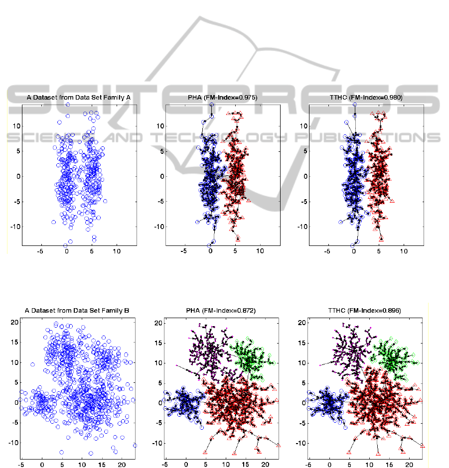
Figure 1: The clustering results and the tree structures produced by PHA and TT_PHA for a dataset from Dataset Family A.
The arrows are used to indicate the parent point, and different symbols are used to show the data points belong to different
clusters.
Figure 2: The clustering results and the tree structures produced by PHA and TT_PHA for a dataset from Dataset Family B.
The arrows are used to indicate the parent point, and different symbols are used to show the data points belong to different
clusters.
MeasuringClusterSimilaritybytheTravelTimebetweenDataPoints
17
Because there are 100 different datasets in each
dataset family, the maximum and the average FM-
Index of the datasets as well as the total running
time in seconds of all the datasets are recorded for
each dataset family. Table 1 shows the results for
Dataset Family A. In terms of the maximum FM-
Index, PHA and TTHC both have produced the
perfect result with FM-Index=1.000, while the
maximum FM-Index produced by the other three
methods is only 0.7045. If the average FM-Index is
concerned, TTHC is the best. Table 2 shows the
results for Dataset Family B. It can be seen that
Ward’s method, PHA and TTHC have produced
better results than the other two methods, while
TTHC has produced the best average FM-Index and
the best maximum FM-Index. For both dataset
families, PHA and TTHC run faster than the other
three methods. Compared to PHA, TTHC has
produced higher average FM-Indices and very
similar maximum FM-Indices. This shows that
TTHC is more robust than PHA for the synthetic
datasets.
To further explain the benefits of using travel
time instead of distance, the results of two datasets
randomly selected from two dataset families are
shown in Figure 1 and Figure 2 respectively. The
trees shown in Figure 1 and Figure 2 represent the
details of the clustering results, which also
correspond to the structure of the data at different
levels. It can be seen that the tree structures
produced by TTHC is different from these produced
by PHA. Compared to the results of PHA, the
directions of the tree edges produced by TTHC are
oriented more towards the cluster centers in both
cases.
Table 1: Experimental results for Dataset Family A.
Method Time
FM-Index
Max Avg
Single
16.03 0.7045 0.7036
Complete
15.82 0.6975 0.5627
Ward’s
17.34 0.6308 0.5413
PHA
10.44 1.0000 0.8126
TTHC
10.94 1.0000 0.8335
Table 2: Experimental results for Dataset Family B.
Method Time
FM-Index
Max Avg
Single
149.82 0.5852 0.5820
Complete
149.57 0.8857 0.6398
Ward’s
154.83 0.9340 0.8433
PHA
41.50 0.9347 0.8855
TTHC
43.16 0.9348 0.8947
4.2 Experiments with Two Real
Datasets
Two real datasets, Iris and Yeast from UCI Machine
Learning Repository (Frank et al., 2010) are also
selected to evaluate the clustering methods. They are
both labeled datasets, so the benchmarks are also
available. The FM-indices and the running time in
seconds for the two datasets are shown in Table 3.
TTHC has produced the best results for both
datasets. For the Iris dataset, TTHC produces a FM-
Index of 0.9234. The dendrogram produced by
TTHC for the Iris dataset is shown in the Appendix
as well. It is found that only 6 out of 150 points in
Iris are assigned incorrectly by TTHC. However, for
the Yeast dataset having 8 attributes, although TTHC
has produced the best FM-Index, it is still a very
poor result because the FM-Index is as low as
0.4713. The result indicates that the Euclidean
squared distance measure used may not be a proper
distance measure for the Yeast dataset. So, a better
distance measure needs to be found and further work
needs to be done in order to apply TTHC method to
high dimensional datasets such as Yeast.
5 CONCLUSION
AND DISCUSSION
We have proposed a new similarity measure for
hierarchical clustering by introducing a hypothetical
travel time between data points. Compared with four
other methods, the resulting TTHC method produces
competitive and promising results when applied to
different datasets. For two data points, if the
difference between the potential values of them
becomes larger, the travel time between them
becomes shorter, and the similarity between them
becomes larger. Close to the border areas of the
clusters in a dataset, the potential difference between
the data points from different clusters are usually
smaller than the potential difference between the
data points from a same cluster, while distances
between them are similar. So using the travel time
can usually increase the similarities between the data
points within a same cluster, while decreasing the
similarities between the data points from different
clusters. This may explain why using the travel time
instead of the distance between data points can
improve the quality of clustering. We also noticed
the limitation of the TTHC method when applied to
a high dimensional dataset. In future work, we plan
to improve the distance measure and to explore
ICPRAM2014-InternationalConferenceonPatternRecognitionApplicationsandMethods
18
different methods for dealing with high dimensional
data.
Table 3: Experimental results for two real datasets.
Method
Iris Yeast
Time
FM-
Index
Time
FM-
Index
Single
0.020 0.7635 9.929 0.4700
Complete
0.015 0.7686 10.091 0.3160
Ward’s
0.018 0.8222 10.248 0.2689
PHA
0.020 0.8670 1.439 0.4694
TTHC
0.020 0.9234 1.468 0.4731
ACKNOWLEDGEMENTS
This work is supported by the National Science
Foundation of China (Grants No. 61272213).
REFERENCES
Assent, I., Clustering high dimensional data, WIREs Data
Mining and Knowledge Discovery, 2: 340–350, 2012.
Endo, Y., Iwata, H., Dynamic clustering based on
universal gravitation model, Modeling Decisions for
Artificial Intelligence, Lecture Notes in Computer
Science, 3558: 183–193, 2005.
Filippone, M., Camastra, F., Masulli, F., Rovetta, S., A
survey of kernel and spectral methods for clustering,
Pattern Recognition, 41(1): 176-190, 2008.
Fowlkes, E.B., Mallows, C.L., A method for comparing
two hierarchical clusterings, Journal of the American
Statistical Association, 78: 553-569, 1983.
Frank, A., Asuncion, A., UCI Machine Learning
Repository [http://archive.ics.uci.edu/ml], 2010.
Irvine, CA: University of California, School of
Information and Computer Science.
Gil-García, R., Pons-Porrata, A., Dynamic hierarchical
algorithms for document clustering, Pattern
Recognition Letters, 31: 469–477, 2010.
Gómez, J., Dasgupta, D., Nasraoui, O., A new
gravitational clustering algorithm, In Proceedings of
the 3rd SIAM International Conference on Data
Mining, pages 83–94, San Francisco, CA, USA, May
1-3, 2003.
Jain, A.K., Data clustering: 50 years beyond K-means,
Pattern Recognition Letters, 31: 651–666, 2010.
Li, J., Fu, H., Molecular dynamics-like data clustering
approach, Pattern Recognition, 44: 1721-1737, 2011.
Lu, Y., Wan, Y., PHA: a fast potential-based hierarchical
agglomerative clustering method, Pattern Recognition,
46(5): 1227–1239, 2013.
Lu, Y., Wan, Y., Clustering by sorting potential values
(CSPV): a novel potential-based clustering method,
Pattern Recognition, 45(9): 3512–3522, 2012.
Murtagh, F., Contreras, P., Algorithms for hierarchical
clustering: an overview, WIREs Data Mining and
Knowledge Discovery, 2: 86–97, 2012.
Omran, M.G., Engelbrecht, A.P., Salman, A., An
overview of clustering methods, Intelligent Data
Analysis, 11(6): 583-605, 2007.
Peng, L., Yang, B., Chen, Y., Abraham, A., Data
gravitation based classification. Information Sciences,
179(6): 809-819, 2009.
Shi, S., Yang, G., Wang, D., Zheng, W., Potential-based
hierarchical clustering, In Proceedings of the 16th
International Conference on Pattern Recognition,
pages 272-275, Quebec, Canada, August 11-15, 2002.
Wang, J., Li, M., Chen, J., Pan, Y., A fast hierarchical
clustering algorithm for functional modules discovery
in protein interaction networks, IEEE Transactions on
Computational Biology and Bioinformatics, 8(3): 607-
620, 2011.
Wright, W.E., Gravitational clustering, Pattern
Recognition, 9: 151-166, 1977.
Yu, H., Gerstein, M., Genomic analysis of the hierarchical
structure of regulatory networks, Proc. National
Academy of Sciences of USA, 103(40): 14724–14731,
October, 2006.
MeasuringClusterSimilaritybytheTravelTimebetweenDataPoints
19
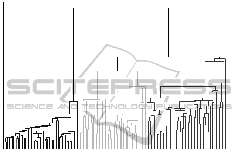
APPENDIX
The Dendrogram Produced by TTHC for the Iris Datase
ICPRAM2014-InternationalConferenceonPatternRecognitionApplicationsandMethods
20
