Detection of Prostate Abnormality within the Peripheral Zone using

Local Peak Information

Andrik Rampun

, Paul Malcolm

and Reyer Zwiggelaar

Department of Computer Science, Aberystwyth University, Aberystwyth SY23 3DB, U.K.

Department of Radiology, Norfolk & Norwich University Hospital, Norwich NR4 7UY, U.K.

Keywords:

Computer Aided Detection of Prostate Cancer, Peak Detection, Prostate Abnormality Detection, Prostate MRI.

Abstract:

In this paper, a fully automatic method is proposed for the detection of prostate cancer within the peripheral

zone. The method starts by ﬁltering noise in the original image followed by feature extraction and smoothing

which is based on the Discrete Cosine Transform. Next, we identify the peripheral zone area using a quadratic

equation and divide it into left and right regions. Subsequently, peak detection is performed on both regions.

Finally, we calculate the percentage similarity and Ochiai coefﬁcients to decide whether abnormality occurs.

The initial evaluation of the proposed method is based on 90 prostate MRI images from 25 patients and 82.2%

(sensitivity/speciﬁcity: 0.81/0.84) of the slices were classiﬁed correctly with 8.9% false negative and false

positive results.

1 INTRODUCTION

In 2013, approximately 239,000 American men were

diagnosed with prostate cancer (more than 20,000 in-

creased compared to 217,730 cases in 2010 (Tempany

and Franco, 2012)). In the United Kingdom, over

40,000 cases are reported annually with more than

10,000 deaths (PCUK, 2013). Generally, there are

several well known clinical diagnostic tests such as

prostate-speciﬁc-antigen (PSA) level (Brawer, 1991),

digital rectal examination (DRE) (Shirley and Brew-

ster, 2011), transrectal ultrasound (TRUS) (Aus et al.,

2008) and biopsy tests (Roehl et al., 2002). Nevethe-

less, prostate cancer too often goes undetected as the

sensitivity and speciﬁcity of these techniques could be

improved and could have complications (Tidy, 2013;

Kenny, 2012; Choi et al., 2007; Tempany and Franco,

2012). Prostate magnetic resonance imaging (MRI)

can provide non-invasive imaging and in combina-

tion with computer technology can provide a detec-

tion tool which has the potential to improve the ac-

curacy of clinical diagnostic tests (Ampeliotis et al.,

2007). Figure 1 shows an example prostate MRI im-

age with its ground truth delineated by an expert radi-

ologist.

This research aims to develop a computer aided

diagnosis (CAD) tool for prostate cancer by compar-

ing data peaks between the left and right regions of

the peripheral zone (PZ). Peak detection methods are

Figure 1: The ground truth of prostate gland, central zone

and tumor are represented in red, yellow and green, respec-

tively.

popular in many signal processing applications. How-

ever, not much work has been done applying such

technique to the detection of prostate cancer based

on MRI analysis. Limited number of methods in

the literature attempted to use peak values in detect-

ing prostate abnormality such as (Vos et al., 2010),

(Reinsberg et al., 2007) and (Choi et al., 2007). A

method proposed by (Vos et al., 2010) uses a peak

detector to select abnormal regions from the obtained

likelihood map constructed during the voxel classiﬁ-

cation stage. Subsequently, they perform automatic

normalisation and histogram analysis for each of the

abnormal regions before calculating malignancy us-

ing a supervised classiﬁer. On the other hand, (Reins-

berg et al., 2007) uses peaks information together

with a apparent diffusion coefﬁcient map to detect

abnormality within the prostate. Another study by

(Choi et al., 2007) shows that peak infromation has

510

Rampun A., Malcolm P. and Zwiggelaar R..

Detection of Prostate Abnormality within the Peripheral Zone using Local Peak Information.

DOI: 10.5220/0004762905100519

In Proceedings of the 3rd International Conference on Pattern Recognition Applications and Methods (ICPRAM-2014), pages 510-519

ISBN: 978-989-758-018-5

 2014 SCITEPRESS (Science and Technology Publications, Lda.)

the potential to improve the detection of prostate can-

cer in MR spectroscopy. In fact, it also allows detec-

tion of prostate cancer in the transitional zone. On the

other hand, (Ampeliotis et al., 2007) used a combined

feature vectors from MRI T-2 weighted images and

Dynamic Contrast Enhanced (DCE) to increase the

sensitivity of prostate cancer detection. (Engelbrecht

et al., 2010) suggests new techniques such as dynamic

contrast-enhanced MRI, diffusion-weighted imaging,

and magnetic resonance spectroscopic imaging yield

signiﬁcant improvements in identiﬁcation and volume

estimation.

In this paper we propose a new method for detect-

ing prostate abnormality within the peripheral zone

based on peak information obtained from the ex-

tracted features. In contrast to the existing methods

in the literature, our method is different in the sense

that:

1. The proposed method does not use any super-

vised/unsupervised classiﬁers for likelihood clas-

siﬁcation of each region as used in (Vos et al.,

2010) and (Ampeliotis et al., 2007).

2. We only used a single modality for abnormal-

ity detection which is T2-Weighted MRI. The

method in (Engelbrecht et al., 2010) used mul-

timodality such as diffusion MRI and MR Spec-

troscopy. Similarly, the method proposed in

(Vos et al., 2010) used a multiparametric MR

of T1- and T2-weighted imaging. (Choi et al.,

2007) suggests that various techniques such as

dynamic contrast materialenhanced MR imag-

ing, diffusion-weighted imaging, and MR spec-

troscopy has the potential to improve the detec-

tion of prostate cancer. On the other hand (Reins-

berg et al., 2007) combined the use of diffusion-

weighted MRI and 1H MR Spectroscopy.

3. The proposed method is purely based on peak in-

formation obtained from extracted features. Un-

like the method in (Vos et al., 2010) they used

additional clinical diagnostic information such as

biopsy tests in making decision as whether cancer

is truly present or not.

2 PROSTATE MODELLING

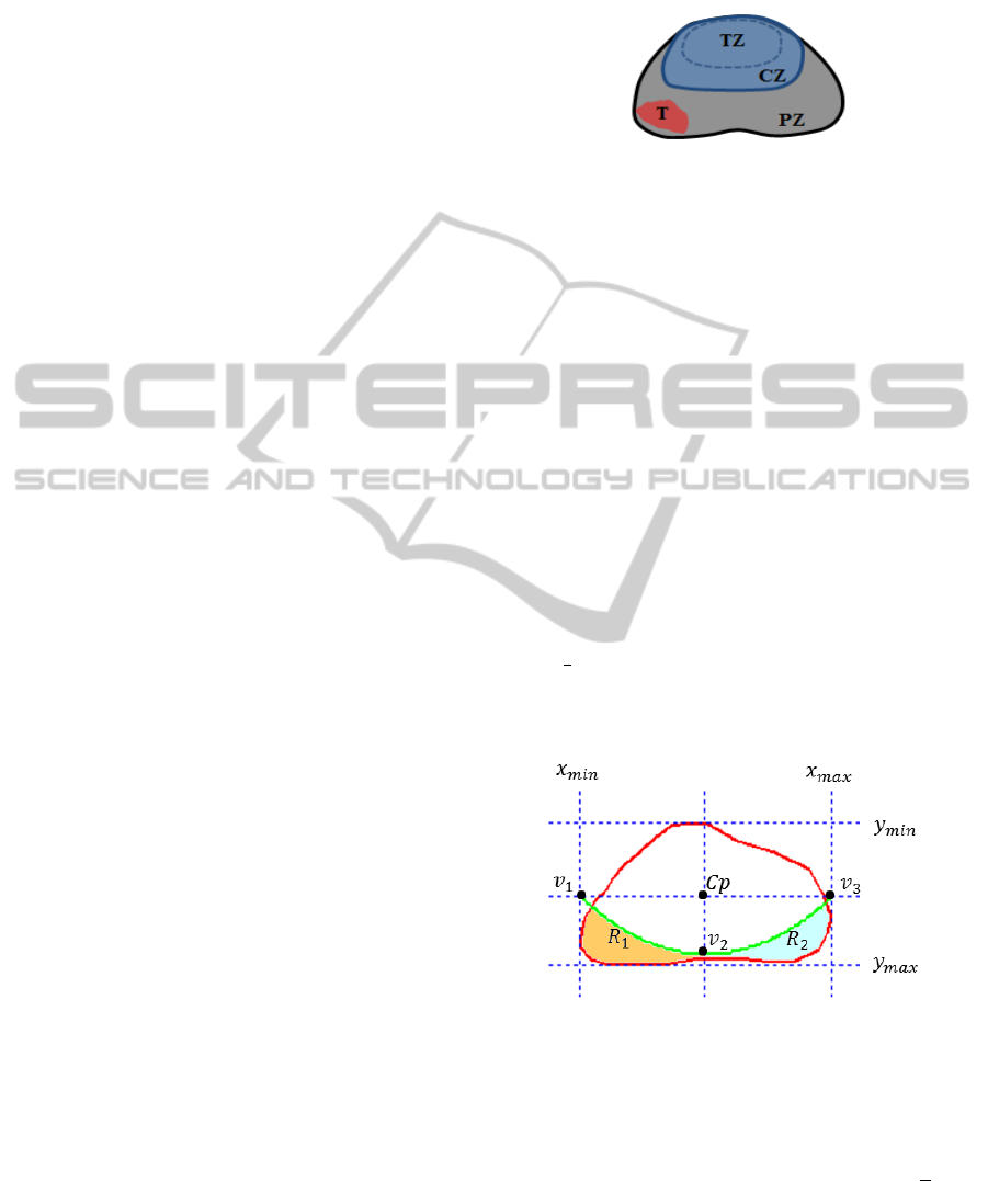
Figure 2 shows a schematic overview of the prostate.

Approximately 70% of prostate cancer can be found

within the peripheral zone (PZ) and 30% within the

central zone (CZ) and transitional zone (TZ) (Choi

et al., 2007). Therefore, this method aims to de-

tect prostate abnormality only within the PZ. We did

not perform automatic prostate segmentation and the

prostates associated regions were delineated by an ex-

pert radiologist.

Figure 2: CZ = central zone, PZ = peripheral zone, TZ =

transitional zone, T = tumor.

Based on the schematic overview shown in Figure

2, we deﬁned our 2D prostate model in Figure 3. The

prostate model has been recently proposed by (Ram-

pun et al., 2013a). The prostate’s PZ is deﬁned us-

ing the quadratic equation y = ax

+ bx + c based on

three crucial coordinate points of the prostate which

are v

and v

. They are determined by the outmost

x and y coordinates of the prostate boundary which are

min

max

min

max

(see Figure 3). For example, x

min

and y

max

can be determined by taking the minimum

and maximum x and y coordinates along the prostate

boundary. Moreover, the x coordinates of v

and v

are captured from x

min

and x

max

and their y coordi-

nate is determined by taking the middle y coordinate

between y

min

and y

max

. On the other hand, the coor-

dinate of v

is taken from the middle x coordinate of

min

and x

max

and its y coordinate is determined by

taking

of the distance from y

min

to y

max

. Mathemat-

ically, these can be represented in equations (1), (2),

(3) and (4).

Figure 3: Prostate gland (red) and the deﬁned PZ below

y = ax

+ bx + c (green) which goes through v

and v

= ((x

min

+ x

max

)/2,(y

min

+ y

max

)/2) (1)

= (x

min

,(y

min

+ y

max

)/2) (2)

= ((x

min

+ x

max

)/2,y

min

+ ((y

max

− y

min

) ×

))

(3)

= (x

max

,(y

min

+ y

max

)/2) (4)

where C

is the central point of the prostate. Once

the coordinates of v

and v

are deﬁned, we can

DetectionofProstateAbnormalitywithinthePeripheralZoneusingLocalPeakInformation

511

determine the values of a, b and c (therefore a ﬁnal

quadratic equation is deﬁned). Finally, by taking ev-

ery x coordinate from x

min

to x

max

into quadratic equa-

tion we are able to determine the y coordinate which

will deﬁne the boundary of R

and R

. R

(amber re-

gion) and R

(turquoise region) are represented by left

and right regions, respectively. By comparing the in-

formation obtained from R

and R

we estimate the

presence of abnormalities.

3 PROPOSED METHODOLOGY

In summary, the proposed methodology starts by ex-

tracting two features from the original image followed

by smoothing each of the extracted features. Subse-

quently, we performed peak detection within R

and

for both features. Finally, based on the peak infor-

mation obtained, a decision is made as to whether an

abnormality is present.

3.1 Features

In many image analysis techniques, features repre-

senting speciﬁc image aspects are important in cap-

turing information representing all textures. This pro-

cess can be done using several techniques such as Ga-

bor Filters (Zheng et al., 2004) (Jain and Karu, 1996),

Grey Level Co-occurence Matrix (GLCM) (Haralick

et al., 1973) (Soh and Tsatsoulis, 1999) (Clausi, 2002)

and Local Binary Pattern (LBP) (Lahdenoja et al.,

2005). According to (Edge et al., 2010) and (Halpern

et al., 2002) most prostate cancers in the PZ tend to

have a dark appearance and several studies suggested

that prostate cancer tissues tend to appear darker on a

T2-weighted MRI image (Garnick et al., 2012) (Ginat

et al., 2009) (Bast et al., 2000). In fact, radiologists

also tend to use darker regions to identify abnormal-

ity within the PZ (Taneja, 2004). In another study

(Vos et al., 2010) showed a potential method to detect

prostate cancer by using blob and peak detectors on

dark blob-like regions within apparent diffusion coef-

ﬁcient (ADC) map. This section presents our features

which are based on low intensities to capture cancer-

ous tissues followed by peak detection which will be

explained in the next section.

In the proposed method, before features are ex-

tracted we performed noise reduction using median

ﬁltering. Median ﬁltering takes the median intensity

value of the pixels within the window as an output in-

tensity of the pixel being processed. We used median

ﬁltering as it can smooth pixels whose values differ

signiﬁcantly from their surroundings without affect-

ing the other pixels (Ekstrom, 1984). Subsequently,

we extracted two features which are f

low

and f

di f

Firstly, f

low

is calculated based on a sum of two vec-

tors (McAllister and Bellittiere, 1996) which can be

computed using

low

(p,q) =

∑

b=1



)

+ (i

)

(5)

where i

is the intensity values of the b

neighbour, i

is the intensity value of the central pixel and f

low

(p,q)

represents a new intensity value at position (p,q). In

addition, N is the number of neighbours which have

intensity values less than the intensity value of the

central pixel. This means, f

low

represents the average

of the sum vector of the central pixel with each of its

neighbours which have lower intensity value than the

central pixel. f

low

contains most of the low intensities

(higher probobality of cancer). In order to extract the

feature we run a small 5 × 5 sliding window over the

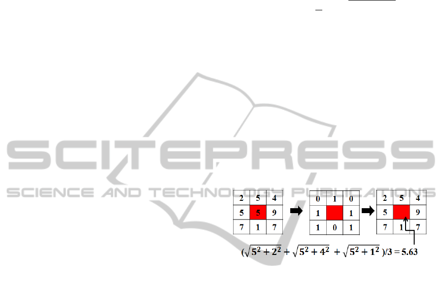
original image (I). Figure 4 shows an example of how

low

(p,q) is calculated for a 3 × 3 window.

Figure 4: f

low

(p,q) is calculated using equation (5) by tak-

ing only those neighbours which have a value smaller than

the central pixel.

On the other hand, the second feature ( f

di f

) is cal-

culated by substracting f

min

from each of the elements

in f

low

. This means, f

di f

contains the information

difference between the sum vector and the minimum

value. f

min

can be calculated by taking the minimum

value within a window.

min

(p,q) = min

{

g(k, l)

}

(6)

where g is a window, g(k, l) ∈ I, I is the original im-

age and k and l is the dimension of the window used.

Once f

min

is extracted we calculate f

di f

using the fol-

lowing the equation

di f

(p,q) = f

low

(p,q) − f

min

(p,q) (7)

This means, f

di f

contains the difference between f

low

and f

min

. f

di f

represents lower intensities than hte

ones in f

low

(this will enhance our chance to capture

more cancerous tissues). For example, based on Fig-

ure 4 f

min

(p,q) = 1 and f

low

(p,q) = 5.63, therefore

di f

(p,q) = 4.63. Since we have two features ( f

low

and f

di f

) for each region R

and R

, from now on we

use R

and R

to //represent R

and R

for each fea-

ture, where r ∈

{

low,di f

}

. Figure 5 shows examples

ICPRAM2014-InternationalConferenceonPatternRecognitionApplicationsandMethods

512

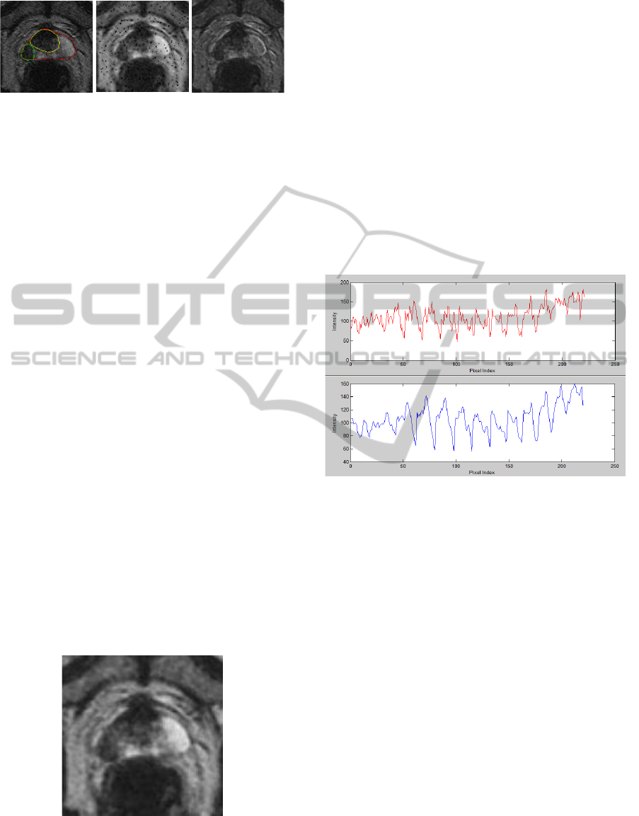
Figure 5: From left is original image, f

low

and f

di f

, respec-

tively.

of features extracted from I. Note that, many black

spots appeared in f

low

. This is due to the effect in

(5) (e.g. if i

is smaller than all of its neighbours val-

ues). Since this will affect the peak detection results,

smoothing/noise reduction is necessary to reduce this

problem.

3.2 Feature Smoothing

According to (Hardle, 1991), feature smoothing is a

process to minimise noise in an image while keeping

the most important aspects of a dataset. In the pro-

posed algorithm, we used two-stage noise reduction

(Rampun et al., 2013b) based on a discrete cosine

transform (DCT) followed by replacement of each

pixel by the average of the neighbouring pixel values

(using a 5 × 5 window). The complete explanation

of DCT can be found in (Cabeen and Gent, 2012).

Despite its good performance, DCT does not spec-

ify Q (the amount of smoothing/compression) auto-

matically (Watson, 1993), which mainly affects the

ﬁnal result of the smoothed image. Garcia’s modi-

ﬁed method (Garcia, 2010) (based on DCT) uses a

smoothing parameter that minimises the generalized

cross-validation (GCV) score to estimate the amount

of smoothing carried out in order to avoid over- or

under-smoothing. Finally, Garcia’s method is robust

in dealing with weighted, missing, and outlien values

by using an iterative procedure (Garcia, 2010). Figure

6 shows an example of f

low

after smoothed.

Figure 6: Smoothed f

low

using DCT. Note that the small

black spots/region (Figure 5) have disappeared.

3.3 Peak Detection

Peak detection is the process of ﬁnding local max-

ima and minima of a signal that satisfy certain proper-

ties (Instruments, 2013). Even though peak detection

is less popular in medical image analysis, there are

numerous methods have been developed particularly

in signal processing (Latha et al., 2011). In signal

processing, peak detection is widely used to capture

signal ﬂuctuation by measuring its properties such as

positions, heights and widths. A common way to per-

form this technique is to make use of the fact that the

ﬁrst derivative of a peak has a downward-going zero-

crossing at the peak maximum. Figure 7 shows an ex-

ample of f

low

within R

before and after smoothing.

In the proposed method we applied peak detection in-

Figure 7: Unsmooth and smoothed signal represents in red

and blue line, respectively. Fewer peaks are detected within

the smoothed signal (blue) which is basically reduce the

number of false zero-crossing.

dividually within R

and R

for each of the features.

Since we are using Ochiai coefﬁcient (Ochiai, 1957)

to measure the similirity between two sets of vectors,

we need to vectorise R

and R

(

⃗

and

⃗

, respec-

tively) by taking each element from top to bottom, left

to right. Each element in

⃗

will be compared to its

neighboring values. If an element is larger than both

of its neighbors, the element is a local peak (Math-

Works, 2013). Mathematically, a peak is deﬁned as

⃗

(p,q) >

⃗

(p,q+1) and

⃗

(p,q) >

⃗

(p,q−1).

This is the same for in

⃗

(p,q).

3.4 Abnormality Detection

In the proposed method, abnormality detection is per-

formed by comparing the peak information obtained

from

⃗

and

⃗

. We calculated the following infor-

mation

1. The Ochiai coefﬁcient(O

) (Ochiai, 1957) be-

tween

⃗

and

⃗

which is similar to the cosine

DetectionofProstateAbnormalitywithinthePeripheralZoneusingLocalPeakInformation

513

similarity (Zhu et al., 2010). The Ochiai coefﬁ-

cient measures the similirity between two sets of

vectors. In principle, any type of similarity co-

efﬁcient can be used, however we chose Ochiai

coefﬁcient because several experiments (Abreu

et al., 2006) (Abreu et al., 2009) have shown that

its performance is better than some other coefﬁ-

cient (Hofer and Wotawa, 2012) such as Tarantula

(Jones and Harrold, 2005) and Jaccard (Yue and

Clayton, 2005). The Ochiai coefﬁcient indicates,

the higher the value the more similar the elements

⃗

and

⃗

which lead to a lower possibility of

the prostate being abnormal.

2. The percentage (S) of elements in

⃗

di f

that fall

within the range of elements in

⃗

di f

(if

⃗

di f

⃗

di f

). The higher the percentage the lower the

difference between

⃗

di f

and

⃗

di f

which means a

lower possibility of the prostate being abnormal.

We will explain how each of the above metrics is cal-

culated in this section. The Ochiai coefﬁcient is de-

ﬁned as

O =

#(A ∩B)



(#(A) ×#(B))

(8)

where A and B are sets which are represented as vec-

tors and #(A) and #(B) are the number of elements in

A and B, respectively. However, since the values in

⃗

and

⃗

are real values (e.g. 3.123) it is impossi-

ble to calculate #(A ∩ B). On the other hand, we only

take elements in

⃗

which are within the minLimit

and maxLimit of each vector. This means, peaks with

values outside the range will be ignored to ensure that

we are considering only realiable peaks and minimise

the effect of noise. We summarise each step for

⃗

low

1. Find the range of

⃗

low

and

⃗

low

range

= max



⃗

low



− min



⃗

low



(9)

where max and min are the maximum and mini-

mum values in

⃗

low

. Assuming that,

⃗

low

has the

smaller range value.

2. Since

⃗

low

has a smaller range, ﬁnd its minLimit

and maxLimit values (if

⃗

low

has smaller range,

ﬁnd its minLimit and maxLimit values instead).

minLimit

⃗

low

= µ

⃗

low

− σ

⃗

low

(10)

maxLimit

⃗

low

= µ

⃗

low

+ σ

⃗

(11)

⃗

low

∑

⃗

low

(p,q) (12)

⃗

low



∑

(

⃗

low

(p,q) −µ

⃗

low

) (13)

where µ and σ represent the mean and standard

deviation of

⃗

low

3. Calculate the Ochiai coefﬁcient using

⃗

low

≤

⃗

low

≤

⃗

low

)



(#(

⃗

low

) ×#(

⃗

low

))

(14)

where #(

⃗

≥

⃗

≤

⃗

) represents the number

of elements in

⃗

which is within minLimit

⃗

and maxLimit

⃗

The steps are the same for the second feature ( f

di f

)

⃗

di f

. Next, we calculate S (the maximum value is

100) using

S =

#((

⃗

≥

⃗

≤

⃗

)

× 100 (15)

where

H =



⃗

di f

, i f #

⃗

di f

> #

⃗

di f

⃗

di f

, otherwise

(16)

The decision whether abnormality is present or

not is based on the ﬂow chart in Figure 8.

Figure 8: Flow chart decision rule.

Based on the conditions above, it shows that a

slice is malignant if both O

low

and O

di f

are smaller

than the threshold value (we selected this parame-

ter value as 0.43 as this produced the highest correct

classiﬁcation rate based on 101 different thresholds

tested (see Figure 14)) or if O

low

or O

di f

are below

the threshold value and S below 60 (we chose this pa-

rameter value as it produced the highest accuracy of

≈ 70% based on 10 different thresholds (10 to 100)

ICPRAM2014-InternationalConferenceonPatternRecognitionApplicationsandMethods

514

tested. The experiment was performed by classifying

every single case using a single S value and selecting

the one with the highest classiﬁcation rate. This ex-

periment is exactly the same when selecting the value

of O

low

and O

di f

). This means, if any of O

low

di f

value is smaller than the threshold, we will use

S to determine the occurance of abnormalities. Nev-

ertheless, if S = 100, we do not have a need to check

because it indicates the maximum similarity per-

centage. Finally, if the third condition in Figure 8 is

passed then the slice is considered benign.

4 EXPERIMENTAL RESULTS

This section presents our experimental results. In to-

tal, our database contains 90 prostate T2-Weighted

MRI images (512 × 512) from 25 different patients

aged 54 to 74. Each patient has 3 to 5 slices through

the central part of the prostate. The prostates, cancer

and central zones were delineated by an expert radi-

ologist on each of the MRI images. Data was anal-

ysed and classiﬁed as to whether the prostate con-

tains cancer based on the conditions explained pre-

viously. Subsequently, we compared the result with

the ground truth whether the prostate contains cancer

regions or not. We will present two different cases

and the justiﬁcation for the threshold values selec-

tion. The ﬁrst case (Figure 9) shows the results of

a slice with cancer. Figure 9 shows the original image

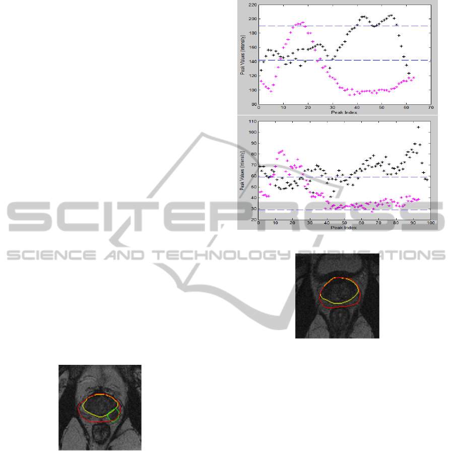
Figure 9: Case # 1: Malignant.

(top) with ground truth, prostate gland (red), CZ (yel-

low) and tumor (green). Figure 10 shows results of

⃗

low

and

⃗

di f

, respectively. Black and magenta rep-

resent

⃗

and

⃗

. On the other hand, maxLimit

⃗

and minLimit

⃗

are represented in the lines which are

parallel with the x axis (broken lines). Note that we

use the same order and notations for the second case

as well. From Figure 10 we can visually identify that

most values in

⃗

and

⃗

are quite separated in both

features. By calculating the matrics deﬁned in section

3.4, we will get the following results: O

low

= 0.177,

di f

= 0.367 and S = 35.71%. Therefore the slice is

considered malignant based on the conditions shown

Figure 10: Results of case # 1: Malignant.

Figure 11: Case # 2: Benign.

in section 3.4.

On the other hand, Figures 11 and 12 show an ex-

ample of a slice without an abnormality and its re-

sults, respectively. In this example, we can see that

≈ 95% of the values in

⃗

and

⃗

are within the same

range (Figure 12). By calculating the metrics we will

get the following results: O

low

= 0.77, O

di f

= 0.81

and S = 72.44%. Therefore, the slice is considered

benign because all metric values are above the thresh-

old values.

Figure 13 shows the Receiver Operating Charac-

teristic (ROC) curves of the proposed method based

on 101 different threshold values. The minimum and

maximum threshold values are 0 and 1, respectively

with 0.01 difference between threshold values. The

ROC graph shows that the proposed method achieved

0.80 true positive rate with 0.20 false positive rate.

In terms of correct classiﬁcation rate (CCR) against

different thresholds, Figure 14 shows that O

< 0.43

achieved the highest CCR of 82.2%. On the other

hand, Figure 14 shows the boxplot of O

low

and O

di f

for benign (blue) and malignant (red) cases. Based on

the results in Figure 14, it is clearly shows that most

DetectionofProstateAbnormalitywithinthePeripheralZoneusingLocalPeakInformation

515

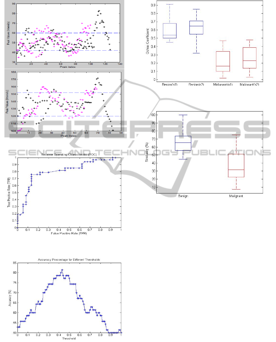
Figure 12: Results of case # 2: Benign.

Figure 13: ROC curves of the proposed method using 101

different threshold values (O

Figure 14: Accuracies of the proposed method using 101

different threshold values (O

benign cases have O

> 0.4 between

⃗

and

⃗

Similarly the results in Figure 15 shows that most be-

Figure 15: O

l ow

and O

di f

represented in o1 and o2, respec-

tively.

Figure 16: Similarity percentage (S) (between

⃗

and

⃗

)

for benign and malignant cases represented in blue and red,

respectively.

nign cases have S > 60 compared to malignant cases

which have S < 60.

For the 90 prostate MRI slices from 25 different

patients (41 slices are malignant and 49 slices are be-

nign), the proposed method achieved 82.2% (74 slices

classiﬁed correctly). On the other hand, the proposed

method produced 8.9% false negative and false posi-

tive results. Since, the number of methods which uses

peak detection methods (in medical image analysis

applications) in the literature is limited, it is hard to

make a direct comparison with other methods. In ad-

dition, different datasets and frameworks used in the

literature also make it extremely difﬁcult to perform

a qualitative comparison. However, to compare our

results indirectly with some existing methods we cite

several methods which have a similar goal (detecting

prostate abnormality/cancer).

Table 1 presents the experimental results of ten

different methods (included our method) and their

average accuracies. Note that every method used

different datasets, modalities and frameworks. The

ICPRAM2014-InternationalConferenceonPatternRecognitionApplicationsandMethods

516

Table 1: First, second and third column represents the au-

thors, number of prostates and average accuracy (AA), re-

spectively.

Authors # of cases AA (%)

(Sung et al., 2011) 42 89

(Vos et al., 2010) 29 89

(Reinsberg et al., 2007) 42 87

(Rampun et al., 2013a) 19 85

(Ampeliotis et al., 2007) 10 84

Our method 25 82

(Castaneda et al., 2009) 15 80

(Litjens et al., 2011) 188 79

(Tiwari et al., 2007) 14 78

(Llobet et al., 2007) 303 62

methods proposed by (Sung et al., 2011) and (Vos

et al., 2010) achieved the highest average accuracy of

89% whereas the methods by (Llobet et al., 2007),

(Tiwari et al., 2007), (Litjens et al., 2011) failed

to achieve more than 80% accuracy. On the other

hand, the proposed method achieved 0.81 sensitiv-

ity and 0.84 speciﬁcity which is similar with the re-

cent method proposed by (Artan and Yetik, 2012).

(Girouin et al., 2007) reports sensitivity/speciﬁcity

value of 0.5-0.6 and 0.13-0.21 over 46 patients us-

ing only T2-weighted (1.5 T) MRI. Further, (Girouin

et al., 2007) presents a higher both sensitivity and

speciﬁcity 0.83 for the same number of patients us-

ing T2-weighted (3.0 T) MRI. In a smaller dataset

(Ftterer et al., 2006) presents 0.83 both on sensitivity

and speciﬁcity, respectively. In a different modality,

(Wong and Scharcanski, 2011) shows a higher sen-

sitivity (0.93) and speciﬁcity (0.96) in 46 ultrasound

images. As mentioned earlier, these comparisions are

very subjective as accuracy, sensitivity and speciﬁcity

are highly inﬂuenced by the number of datasets, dif-

ferent modalities and methods’ frameworks. There-

fore it is extremely difﬁcult to make a real compar-

ison either quantitatively or qualitatively. Some ob-

vious drawbacks of the proposed method, it failed to

produce accurate results in two cases: a) when the

prostate’s peripheral zone is almost non-existent, and

b) when the prostate’s shape does not conform to the

shape of our prostate model.

5 CONCLUSIONS

The proposed method shows that peak information

has a potential role in detecting prostate abnormalities

within the PZ. In contrast with some of the methods

in Table 1, our method uses a minimal set of features

and modalities (only T2-Weighted MRI). Methods by

(Engelbrecht et al., 2010) and (Vos et al., 2010) used

multimodalities data such as diffusion MRI, MR spec-

troscopy and a combination of T1 and T2-weighted

imaging. Secondly, the proposed method does not

use any supervised/unsupervised classiﬁers for clas-

siﬁcation but it is entirely dependent on the metric

values computed from the peak information. More-

over, our method does not refer to or use any clinical

features in making decision as to whether abnormal-

ity occurs but is entirely based on the values of O

and S. The method of (Vos et al., 2010) used clinical

features such as PSA level to support their method in

making decision whether abnormality is truly present

or not. Nevertheless, one obvious drawback of our

method is that it does not have an additional method to

reduce false positive and false negative results. There-

fore a robust false positive/negative reduction method

is needed to increase the accuracy rate. Secondly, if

the tumor appears outside the R

and R

regions the

method failed to identify the abnormality due to the

incorrect information captured. To solve this issue,

we are developing a segmentation method to sepa-

rate CZ from prostate gland. This allows the proposed

method to be more robust because it will analyse re-

gions within the prostate (therefore improving the 2D

PZ model will be apart of our future work).

In short, with 8.9% false negative and false pos-

itive results (sensitivity/speciﬁcity: 0.81/0.84), the

proposed method achieved similar accuracy with

some of the methods in the literature. In our study, we

have shown that most MRI slices containing cancer

have small value of Ochiai coefﬁcient (O

< 0.43)

and S < 60%. This means, if the coefﬁcient be-

tween

⃗

and

⃗

is less than a threshold value (in

our case 0.43), the prostate has a higher probability

to be abnormal. Moreover, a similarity percentage

less than 60% also indicate prostate abnormality. Fi-

nally, the next stage of this research is to test the pro-

posed method on a larger dataset with a combination

of several methods (e.g. CZ segmentation, false pos-

itive/negative reduction, and blob detection), improv-

ing the 2D PZ model and other statistical features (e.g.

entropy and energy).

REFERENCES

Abreu, R., Zoeteweij, P., Golsteijn, R., and van Gemund,

A. J. (2009). A practical evaluation of spectrum-based

fault localization. Journal of Systems and Software,

82(11):1780 – 1792. ¡ce:title¿SI: {TAIC} {PART}

2007 and {MUTATION} 2007¡/ce:title¿.

Abreu, R., Zoeteweij, P., and Van Gemund, A. J. C. (2006).

An evaluation of similarity coefﬁcients for software

fault localization. In Dependable Computing, 2006.

DetectionofProstateAbnormalitywithinthePeripheralZoneusingLocalPeakInformation

517

PRDC ’06. 12th Paciﬁc Rim International Symposium

on, pages 39–46.

Ampeliotis, D., Antonakoudi, A., Berberidis, K., and

Psarakis, E. Z. (2007). Computer aided detection of

prostate cancer using fused information from dynamic

contrast enchanced and morphological magnetic res-

onance images. In IEEE International Conference

on Signal Processing and Communications(ICSPC

2007).

Artan, Y. and Yetik, I. (2012). Prostate cancer localiza-

tion using multiparametric mri based on semisuper-

vised techniques with automated seed initialization.

Information Technology in Biomedicine, IEEE Trans-

actions on, 16(6):1313–1323.

Aus, G., Hermansson, C. G., Hugosson, J., and Pedersen,

K. V. (2008). Transrectal ultrasound examination of

the prostate: complications and acceptance by pa-

tients. British journal of urology, 71(4):457–459.

Bast, R. C., Kufe, D. W., Pollock, R. E., Weichselbaum,

R. R., Holland, J. F., Frei, E., Halvorsen, R. A., and

Thompson, W. M. (2000). Imaging neoplasms of the

abdomen and pelvis.

Brawer, M. K. (1991). Prostate specic antigen: A review.

Acta Oncologica., 30(2):161–168.

Cabeen, K. and Gent, P. (2012). Image com-

pression and the Discrete Cosine Transform.

http://www.lokminglui.com/dct.pdf/. Accessed

11-August-2013.

Castaneda, B., An, L., Wu, S., Baxter, L. L., Yao, J. L.,

Joseph, J. V., Hoyt, K., Strang, J., Rubens, D., and

Parker, K. J. (2009). Prostate cancer detection using

crawling wave sonoelastography. In Proc. SPIE 7265,

Medical Imaging 2009: Ultrasonic Imaging and Sig-

nal Processing.

Choi, Y. F., Kim, F. K., Kim, N., Kim, K. W., Choi, E. K.,

and Cho, K.-S. (2007). Functional MR imaging of

prostate cancer. RadioGraphics, 27(1):63–68.

Clausi, D. A. (2002). An analysis of co-occurrence texture

statistics as a function of grey level quantization. Can.

J. Remote Sensing, 28(1):45–62.

Edge, S. B., Byrd, D. R., Compton, C., Fritz, A. G., Greene,

F. L., and Trotti, A. (2010). AJCC Cancer Staging

Manual (7th Edition). Springer., Chicago, US.

Ekstrom, P. M. (1984). Digital Image Processing Tech-

niques. Academic Press, Inc., London, UK.

Engelbrecht, M. R., Puech, P., Colin, P., Akin, O. Lemaitre,

L., and Villers, A. (2010). Multimodality magnetic

resonance imaging of prostate cancer. Journal of en-

dourology society, 24(5):677–684.

Ftterer, J. J., Heijmink, S. W. T. P. J., Scheenen, T. W. J.,

Veltman, J., Huisman, H. J., Vos, P., de Kaa, C.

A. H., Witjes, J. A., Krabbe, P. F. M., Heerschap,

A., and Barentsz, J. O. (2006). Prostate cancer lo-

calization with dynamic contrast-enhanced mr imag-

ing and proton mr spectroscopic imaging. Radiology,

241(2):449–458. PMID: 16966484.

Garcia, D. (2010). Robust smoothing of gridded data in one

and higher dimensions with missing values. Computa-

tional Statistics and Data Analysis, 54(4):1167–1178.

Garnick, M. B., MacDonald, A., Glass, R., and Leighton,

S. (2012). Harvard Medical School 2012 Annual Re-

port on Prostate Diseases. Harvard Medical School,

Harvard , US.

Ginat, D. T., Destounis, S. V., Barr, R. G., Castaneda, B.,

Strang, J. G., and Rubens, D. J. (2009). Us elastog-

raphy of breast and prostate lesions1. Radiographics,

29(7):2007–2016.

Girouin, N., M

ege-Lechevallier, F., Senes, A. T., Bissery,

A., Rabilloud, M., Mar

echal, J., Colombel, M., Ly-

onnet, D., and Rouvi

ere, O. (2007). Prostate dy-

namic contrast-enhanced mri with simple visual diag-

nostic criteria: is it reasonable? European radiology,

17(6):1498–1509.

Halpern, E. J., Cochlin, D. L., and Goldberg, B. (2002).

Imaging of the Prostate. Martin Dunitz Ltd., London,

UK.

Haralick, R. M., Shanmugam, K., and Dinstein, I. (1973).

Textural features for image classiﬁcation. IEEE

Transactions On Systems, Man, and Cybernetics,

3(6):610–621.

Hardle, W. (1991). Smoothing Techniques With Implemen-

tation in S. Springer-Verlag., Louvain-La-Neuve, Bel-

gium.

Hofer, B. and Wotawa, F. (2012). Spectrum enhanced dy-

namic slicing for better fault localization. In ECAI,

pages 420–425.

Instruments (2013). Wavelet-based peak detection.

http://www.ni.com/white-paper/5432/en/. Accessed

24-July-2013.

Jain, A. K. and Karu, K. (1996). Learning texture discrim-

ination. IEEE Transactions on Pattern Analysis and

Machine Intelligence, 18:195–205.

Jones, J. A. and Harrold, M. J. (2005). Empirical evaluation

of the tarantula automatic fault-localization technique.

In Proceedings of the 20th IEEE/ACM International

Conference on Automated Software Engineering, ASE

’05, pages 273–282, New York, NY, USA. ACM.

Kenny, T. (2012). Prostate cancer.

http://www.patient.co.uk/health/prostate-cancer/.

Accessed 12-August-2013.

Lahdenoja, O., Laiho, M., and Paasio, A. (2005). Local bi-

nary pattern feature vector extraction with cnn. In 9th

International Workshop on Cellular Neural Networks

and Their Applications, pages 202–205. IEEE Cat.

Latha, I., Reichenbach, S. E., and Tao, Q. (2011). Compar-

ative analysis of peak-detection techniques for com-

prehensive two-dimensional chromatography. Radio-

Graphics, 1218(38):6792–6798.

Litjens, G. J. S., Vos, P. C., Barentsz, J. O., Karssemeijer,

N., and Huisman, H. J. (2011). Automatic computer

aided detection of abnormalities in Multi-Parametric

prostate MRI. In Proc. SPIE 7963, Medical Imaging

2011: Computer-Aided Diagnosis.

Llobet, R., Juan, C., Cortes, P., Juan, A., and Toselli, A.

(2007). Computer-aided detection of prostate can-

cer. International Journal of Medical Informatics,

76(7):547–556.

MathWorks (2013). Documentation center: ﬁndpeaks.

ICPRAM2014-InternationalConferenceonPatternRecognitionApplicationsandMethods

518

http://www.mathworks.co.uk/help/signal/ref/ﬁndpeaks.html/.

Accessed 23-August-2013.

McAllister, H. C. and Bellittiere, D.

(1996). The sum of two vectors.

http://www.hawaii.edu/suremath/jsumTwoVectors.html.

Accessed 19-August-2013.

Ochiai, A. (1957). Zoo geographical studies on the solenoid

ﬁshes found Japan and its neighboring regions.ii.

Bull.Japan.Soc.Sci.Fisheries., 22(9):526–530.

PCUK (2013). Prostate cancer facts and ﬁgures.

http://prostatecanceruk.org/information/prostate-

cancer-facts-and-ﬁgures/. Accessed 11-August-2013.

Rampun, A., Chen, Z., and Zwiggelaar, R. (2013a). Detec-

tion and localisation of prostate abnormalities. In 3rd

International Conference on Computational & Math-

ematical Biomedical Engineering, CMBE 13.

Rampun, A., Strange, H., and Zwiggelaar, R. (2013b).

Texture segmentation using different orientations of

GLCM features. In 6th International Conference on

Computer Vision / Computer Graphics Collaboration

Techniques and Applications, MIRAGE 13.

Reinsberg, S. A., Payne, G. S., Riches, S. F., Ashley,

S., Brewster, J. M., Morgan, V. A., and deSouza,

N. M. (2007). Combined use of Diffusion-Weighted

MRI and 1H MR Spectroscopy to increase accuracy

in prostate cancer detection. American Journal of

Roentgenology, 188(1):1122–1129.

Roehl, K. A., Antenor, J. A. V., and Catalona, W. J.

(2002). Serial biopsy results in prostate cancer screen-

ing study. British journal of urology, 167(6):2435–

2439.

Shirley, A. and Brewster, S. (2011). Expert review: The

digital rectal examination. Journal of Clinical Exami-

nation, 11:1–12.

Soh, L. and Tsatsoulis, C. (1999). Texture analysis of sar

sea ice imagery using gray level co-occurrence matri-

ces. Geoscience and Remote Sensing, IEEE Transac-

tions on, 37(2):780–795.

Sung, Y. S., Kwon, H.-J., Park, B. W., Cho, G., Lee,

C. K., Cho, K.-S., and Kim, J. K. (2011). Prostate

cancer detection on dynamic contrast-enhanced mri:

Computer-aided diagnosis versus single perfusion pa-

rameter maps. American Journal of Roentgenology,

197(5):1122–1129.

Taneja, S. S. (2004). Imaging in the diagnosis and manage-

ment of prostate cancer. Reviews in Urology, 6(3):101.

Tempany, C. and Franco, F. (2012). Prostate MRI: Update

and current roles. Applied Radiology, 41(3):17–22.

Tidy, C. (2013). Prostate speciﬁc antigen (PSA) test.

http://www.patient.co.uk/health/prostate-speciﬁc-

antigen-psa-test/. Accessed 12-August-2013.

Tiwari, P., Madabhushi, A., and Rosen, M. (2007). A hier-

archical unsupervised spectral clustering scheme for

detection of prostate cancer from magnetic resonance

spectroscopy (MRS). In Medical Image Computing

and Computer Assisted Intervention (MICCAI), pages

278–286.

Vos, P. C., Hambrock, T., Barentsz, J., and Huisman, H.

(2010). Computer-assisted analysis of peripheral zone

prostate lesions using T2-weighted and dynamic con-

trast enhanced T1-weighted MRI. Physics in Medicine

and Biology, 55:1719–1734.

Watson, A. B. (1993). Dctune: A technique for visual op-

timization of dct quantization matrices for individual

images. Society for Information Display Digest of

Technical Papers, XXIV:946–949.

Wong, A. and Scharcanski, J. (2011). Fisher #x2013;tippett

region-merging approach to transrectal ultrasound

prostate lesion segmentation. Information Technology

in Biomedicine, IEEE Transactions on , 15(6):900–

907.

Yue, J. C. and Clayton, M. K. (2005). A similarity mea-

sure based on species proportions. Communications in

Statistics - Theory and Methods, 34(11):2123–2131.

Zheng, D., Zhao, Y., and Wang, J. (2004). Feature extrac-

tion using a gabor ﬁlter family. In Proceedings of

the 6th IASTED International Conference on Signal

and Image Processing. The International Association

of Science and Technology for Development.

Zhu, S., Wu, J., and Xia, G. (2010). Top-k cosine similar-

ity interesting pairs search. In Seventh International

Conference on Fuzzy Systems and Knowledge Discov-

ery (FSKD).

DetectionofProstateAbnormalitywithinthePeripheralZoneusingLocalPeakInformation

519