Applying Machine Learning Techniques to Baseball Pitch Prediction

Michael Hamilton

, Phuong Hoang

, Lori Layne

, Joseph Murray

, David Padgett

, Corey Stafford

and Hien Tran

Mathematics Department, Rutgers University, New Brunswick, New Jersey, U.S.A.

Department of Mathematics, North Carolina State University, Raleigh, North Carolina, U.S.A.

MIT Lincoln Laboratory, Lexington, Massachusetts, U.S.A.

Department of Applied Physics & Applied Mathematics, Columbia University, New York, New York, U.S.A.

Keywords:

Pitch Prediction, Feature Selection, ROC, Hypothesis Testing, Machine Learning.

Abstract:

Major League Baseball, a professional baseball league in the US and Canada, is one of the most popular sports

leagues in North America. Partially because of its popularity and the wide availability of data from games,

baseball has become the subject of signiﬁcant statistical and mathematical analysis. Pitch analysis is especially

useful for helping a team better understand the pitch behavior it may face during a game, allowing the team

to develop a corresponding batting strategy to combat the predicted pitch behavior. We apply several common

machine learning classiﬁcation methods to PITCH f/x data to classify pitches by type. We then extend the

classiﬁcation task to prediction by utilizing features only known before a pitch is thrown. By performing

signiﬁcant feature analysis and introducing a novel approach for feature selection, moderate improvement

over former results is achieved.

1 INTRODUCTION

Baseball is one of the most popular sports in North

America. In 2012, Major League Baseball (MLB)

had the highest season attendance of any American

sports league (MLB, 2012). Partially due to this pop-

ularity and the discrete nature of gameplay (allowing

easy recording of game statistics between plays) and

the long history of baseball data collection, baseball

has become the target of signiﬁcant mathematical and

statistical analysis. Player performance, for example,

is often analyzed so baseball teams can modify their

roster (by drafting and trading players) to achieve the

best possible team conﬁguration.

One area of statistical analysis of baseball that

has gained attention in the last decade is pitch anal-

ysis. To aid this study, baseball pitch data produced

by the PITCH f/x system is now widely available for

both public and private use. This data contains use-

ful information about each pitch; several character-

istics such as pitch speed, break angle, and type are

recorded. Because of the accessibility of large vol-

umes of data, both fans and professionals can perform

their own pitch studies, including sabermetrics anal-

ysis. Related pitch data analysis is available in the

literature. For example, Weinstein-Gould (Weinstein-

Gould, 2009) examines pitching strategy of major

league pitchers, speciﬁcally determining whether or

not pitchers (from a game theoretic approach) im-

plement optimally mixed strategies for handling bat-

ters. The research suggests that pitchers do mix op-

timally with respect to the pitch variable. In an eco-

nomic sense, this means that pitchers behave ratio-

nally relative to the result of any given pitch. An in-

teresting note from the author is that although MLB

pitchers are in the perfect position to utilize optimal

strategy mixing (compared to other research subjects

who have little motivation to optimally mix strate-

gies), “...experience, large monetary incentives, and

a competitive environment are not sufﬁcient condi-

tions to compel players to play optimally.” Knowing

this, we obtain useful information about how pitchers

make decisions and (theoretically) which factors are

more important than others in prediction; by knowing

the results pitchers respond to (and the ones they don’t

respond to), it is possible reverse engineer this in-

formation and correspondingly tweak predictions for

maximal accuracy.

Count (number of balls and strikes in the current

at bat) is often cited as a basis for decisive strategy.

520

Hamilton M., Hoang P., Layne L., Murray J., Padget D., Stafford C. and Tran H..

Applying Machine Learning Techniques to Baseball Pitch Prediction.

DOI: 10.5220/0004763905200527

In Proceedings of the 3rd International Conference on Pattern Recognition Applications and Methods (ICPRAM-2014), pages 520-527

ISBN: 978-989-758-018-5

 2014 SCITEPRESS (Science and Technology Publications, Lda.)

For example, Ganeshapillai and Guttag (Ganeshapil-

lai and Guttag, 2012) show that pitchers are much

more predictable in counts that favor the batter (usu-

ally more balls than strikes). Furthermore, Hopkins

and Magel (Hopkins and Magel, 2008) show a dis-

tinct effect of count on the slugging percentage of the

batter. More speciﬁcally, they show that average slug-

ging percentage is signiﬁcantly lower in counts that

favor the pitcher; however, there is no signiﬁcant dif-

ference in average slugging percentage (a weighted

measure of the on-base frequency of a batter) in neu-

tral counts or counts that favor the batter (Hopkins

and Magel, 2008). These results verify that count has

a signiﬁcant effect on the pitcher-batter relationship,

and will thus be an important factor in pitch predic-

tion. Another interesting topic is pitch prediction,

which could have signiﬁcant real-world applications

and potentially improve batter performance in base-

ball. One example of research on this topic is the work

by Ganeshapillai and Guttag (Ganeshapillai and Gut-

tag, 2012), who use a linear support vector machine

(SVM) to perform binary (fastball vs. nonfastball)

classiﬁcation on pitches of unknown type. The SVM

is trained on PITCH f/x data from pitches in 2008 and

tested on data from 2009. Across all pitchers, an aver-

age prediction accuracy of roughly 70 percent is ob-

tained, though pitcher-speciﬁc accuracies vary.

In this paper we provide a machine learning ap-

proach to pitch prediction, using classiﬁcation meth-

ods to predict pitch types. Our results build upon the

work in (Ganeshapillai and Guttag, 2012); however

we are able to improve performance by examining

different types of classiﬁcation methods and by tak-

ing a pitcher adaptive approach to feature set selec-

tion. For more information about baseball itself, con-

sult the Appendix for a glossary of baseball terms.

2 METHODS

2.1 PITCH f/x Data

Our classiﬁers are trained and tested using PITCH f/x

data from all MLB games during the 2008 and 2009

seasons. Raw data is publicly available (Pitchf/x,

2013), though we use scraping methods to transform

the data into a suitable format. The data contains ap-

proximately 50 features (each represents some char-

acteristic of a pitch like speed or position); however,

we only use 18 features from the raw data and create

additional features that are relevant to prediction. For

example, some created features are: the percentage of

fastballs thrown in the previous inning, the velocity of

the previous pitch, strike result percentage of previous

pitch, and current game count (score). For a full list

of features used, see Appendix.

We apply classiﬁcation methods to the data to pre-

dict pitches. On that note, it is important to clarify

a subtle distinction between pitch classiﬁcation and

pitch prediction. The distinction is simply that clas-

siﬁcation uses post-pitch information about a pitch to

determine which type it is, whereas prediction uses

pre-pitch information to classify its type. For exam-

ple, we may use features like pitch speed and curve

angle to determine whether or not it was a fastball.

These features are not available pre-pitch; in that case

we use information about prior results from the same

scenario to judge which pitch can be expected.

The prediction process is performed as binary

classiﬁcation (see section 2.2); all pitch types are

members of one of two classes (fastball and nonfast-

ball). We conduct prediction for all pitchers who had

at least 750 pitches in both 2008 and 2009. This spec-

iﬁcation results in a set of 236 pitchers. For each

pitcher, the data is further split by each count and,

with 12 count possibilities producing 2,832 smaller

subsets of data (one for each pitcher and count com-

bination). After performing feature selection (see sec-

tion 2.3) on each data subset, each classiﬁer (see Ap-

pendix) is trained on each subset of data from 2008

and tested on each subset of data from 2009. The

average classiﬁcation accuracy for each classiﬁer is

computed for test points with a type conﬁdence (one

feature in the PITCH f/x data that measures the con-

ﬁdence level that the pitch type is correct) of at least

0.5.

2.2 Classiﬁcation Methods

Classiﬁcation is the process of taking an unlabeled

data observation and using some rule or decision-

making process to assign a label to it. Within the

scope of this research, classiﬁcation represents deter-

mining the type of a pitch, i.e. given a pitch x with

characteristics x

, determine which pitch type (curve-

ball, fastball, slider, etc) x is. There are several clas-

siﬁcation methodologies one can use to accomplish

this task, here we used the methods of Support Vec-

tor Machine (SVM) and k−nearest neighbor (k-NN),

they are explained in full detail in (Theodoridis and

Koutroumbas, 2009).

2.3 Feature Selection Methods

The key differences between our approach and former

research (Ganeshapillai and Guttag, 2012) is the fea-

ture selection methodology. Rather than using a static

set of features, a different optimal set of features is

ApplyingMachineLearningTechniquestoBaseballPitchPrediction

521

used for each pitcher/count pair. This allows the algo-

rithm to adapt for optimal performance on each indi-

vidual subset of data.

In baseball there are a number of factors that in-

ﬂuence the pitcher’s decision (consciously or uncon-

sciously). For example, one pitcher may not like to

throw curveballs during the daytime because the in-

creased visibility makes them easier to spot; how-

ever, another pitcher may not make his pitching de-

cisions based on the time of the game. In order to

maximize accuracy of a prediction model, one must

try to accommodate each of these factors. For exam-

ple, a pitcher may have particularly good control of a

certain pitch and thus favors that pitch, but how can

one create a feature to represent its favorability? One

could, for example, create a feature that measures the

pitcher’s success with a pitch since the beginning of

the season, or the previous game, or even the previous

batter faced. Which features would best capture the

true effect of his preference for that pitch? The an-

swer is that each of these approaches may be best in

different situations, so they all must be considered for

maximal accuracy. Pitchers have different dominant

pitches, strategies and experiences; in order to maxi-

mize accuracy our model must be adaptable to various

pitching situations.

Of course, simply adding many features to our

model is not necessarily the best choice because

we leave noise from situationally useless features

and suffer from curse of dimensionality issues. We

change our problem of predicting a pitch into pre-

dicting a pitch for each given pitcher in each given

count. We maximize accuracy by choosing (for each

pitcher/count pair) an optimal pool of features from

the entire available set. This allows us to maintain our

adaptive strategy while controlling dimensionality.

2.3.1 Feature Selection Implementation

As alluded to earlier, our feature selection scheme is

adaptive, ﬁnding a good feature set for each (pitcher,

count), e.g., (Rivera, 0-2). Our adaptive feature selec-

tion approach consists of 3 stages.

1. We create about 80 features (see the full list in the

Appendix). We then group all of our generated

features together into groups by similarity. Such

grouping might contain 4 to 12 similar features

such as accuracy over the last pitch, the last ﬁve

pitches, ten pitches, and accuracy over all pitches

in the last inning, etc.

2. We then compute the Receiver Operating Charac-

teristic (ROC) curve for each group of features,

then select the strongest one or two to move on to

the next stage. In practice, selecting only the best

feature provides worse prediction than selecting

the best two or three features. Hence at this stage,

the size of each group is reduced from 4 to 12 to

2 or 3.

3. We next remove all redundant features from our

ﬁnal feature set. From our grouping, features are

taken based on their relative strength. There is

the possibility that a group of features might not

have good predictive power. In those cases, the

resulting set of features is pruned by conducting

hypothesis testing to measure signiﬁcance of each

feature at the α = .01 level.

For a schematic diagram of our approach, see Figure

Figure 1: Schematic diagram of the proposed features se-

lection.

2.3.2 ROC Curves

The Receiver Operating Characteristic (ROC) curve

are used for each individual feature in order to mea-

sure how useful a feature is in prediction. We cal-

culate this by measuring the area between the single

feature ROC curve and the line created by standard

guessing. This value of area tells us how much bet-

ter the feature is at distinguishing the two classes,

compared to standard guessing. These area values

are in the range of [0, 0.5), where a value of 0 rep-

resents no improvement over random guessing and

0.5 would represent perfect distinction between both

classes. For a more detailed description of the ROC

curve, see (Fawcett, 2006) and also Figure 2.

2.3.3 Hypothesis Testing

The ability of a feature to distinguish between two

classes can be determined using a hypothesis test.

Given any feature f , we compare µ

and µ

, the mean

values of f in Class 1 (fastballs) and Class 2 (nonfast-

balls), respectively. Then we consider

: µ

= µ

(1)

: µ

6= µ

(2)

ICPRAM2014-InternationalConferenceonPatternRecognitionApplicationsandMethods

522

Figure 2: The diagonal line represents the tradeoff between

true positive rate (sensitivity) and false positive rate by ran-

dom guessing. The curve represents a shift in this tradeoff

by using a given feature to assign class labels instead of

randomly guessing. In this case the shift represents an im-

provement in distinction between the two classes and the

region between the curve and line quantiﬁes this improve-

ment.

and conduct a hypothesis test using the student’s t dis-

tribution. We compare the p-value of the test against

a signiﬁcance level of α = .01. When the p-value is

less than α, we reject the null hypothesis and con-

clude that the studied feature means are different for

each class, meaning that the feature is signiﬁcant in

separating the classes. In that sense, this test allows

us to remove features which have insigniﬁcant sepa-

ration power.

3 RESULTS

In this paper, we propose a new technique in the prob-

lem of baseball pitch prediction. Speciﬁcally, we

segment the prediction task by pitcher and count be-

cause each of these situations is different enough that

it would be a mistake to consider them equally. For

prediction by pitcher, we used data from 236 pitchers

(as noted in section 2.1). We then selected eight pitch-

ers from the 2008 and 2009 MLB regular seasons to

examine in details.

Table 1: Data for each pitcher.

Pitcher Training Size Test Size

Fuentes 919 798

Madson 975 958

Meche 2821 1822

Park 1309 1178

Rivera 797 850

Vaquez 2412 2721

Wakeﬁeld 2110 1573

Weathers 943 813

Table 1 describes the training and testing sets.

Data from 2008 season were used for training and

data from 2009 were used for testing. Table 2 depicts

the prediction accuracy among the eight pitchers as

compared across classiﬁers as well as naive guess. On

average, 79.76% of pitches are correctly predicted by

SVM-L and SVM-G classiﬁers while k-NN perform

slightly better, at 80.88% accurate. Furthermore, k-

NN is also a better choice in term of computational

speed, as noted in Table 3.

We compare the results of our prediction model

to a naive model that predicts simply by guessing a

pitcher’s most common pitch (either fastball or non-

fastball) from the training data and compute the im-

provement in accuracy in Table 4. The improvement

factor (percent), I, is calculated as follow:

I =

− A

× 100 (3)

where A

and A

denotes the accuracies of naive guess

and our model accordingly. The naive guess simply

return the most frequent pitch type thrown by each

pitcher, calculated from the training set (Ganeshapil-

lai and Guttag, 2012).

The average prediction accuracy of our model

over all 236 pitchers in 2009 season is 77.45%. Com-

pared to the naive model’s natural prediction accu-

racy, our model on average achieves 20.85% improve-

ment. In previous work (Ganeshapillai and Guttag,

2012), the average prediction accuracy of 2009 sea-

son is 70% with 18% improvement over the naive

model. It should be noted that previous work con-

siders 359 pitchers who threw at least 300 pitches in

both 2008 and 2009 seasons. In our study, we only

consider those pitchers that threw at least 750 pitches

in a season. This reduces the number of pitchers that

we considered to 236 pitchers.

In addition, we demonstrate the prediction accu-

racy of our model for each count situation. As illus-

trated in Figures 3 and 4, prediction accuracy is sig-

niﬁcant higher in batter-favored counts and is approx-

imately equal in neutral and pitcher-favored counts.

We also calculate prediction accuracy for 2012

season, using training data from 2011 season or from

both 2010 and 2011 seasons. We again only select

pitchers who had at least 750 pitches in those seasons.

As shown in Table 5, the average pitch prediction ac-

curacy is about 75% in both cases (even though the

size of training data is double in the second case).

ApplyingMachineLearningTechniquestoBaseballPitchPrediction

523

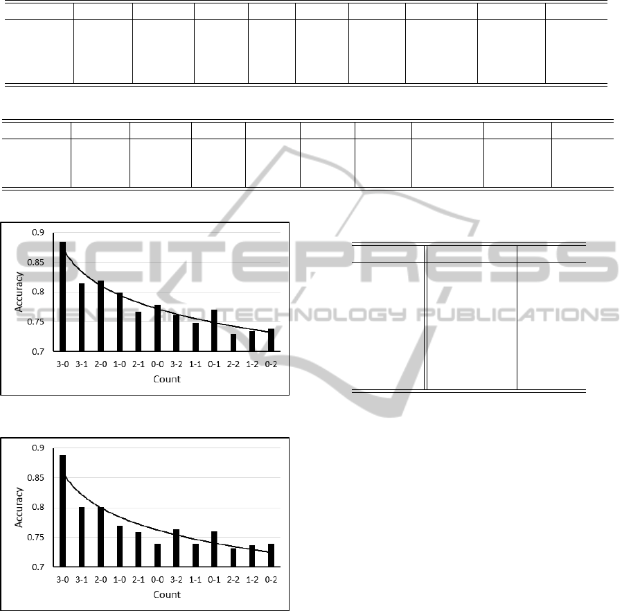
Table 2: Prediction accuracy comparison (percents). Symbols: k-Nearest Neighbors (k-NN), Support Vector Machine with

linear kernel (SVM-L), Support Vector Machine with Gaussian kernel (SVM-G), Naive Guess (NG).

Classiﬁer Fuentes Madson Meche Park Rivera Vaquez Wakeﬁeld Weathers Average

k-NN 80.15 81.85 72.73 70.31 93.51 72.50 100.00 76.01 80.88

SVM-L 78.38 77.23 74.83 72.40 89.44 72.50 95.50 77.76 79.76

SVM-G 76.74 79.38 74.17 71.88 90.14 73.05 96.33 76.38 79.76

NG 71.05 25.56 50.77 52.60 89.63 51.20 100.00 35.55 66.04

Table 3: CPU Times (seconds).

Classiﬁer Fuentes Madson Meche Park Rivera Vaquez Wakeﬁeld Weathers Average

k-NN 0.3459 0.3479 0.3927 0.3566 0.4245 0.4137 0.4060 0.3480 0.3794

SVM-L 0.7357 0.5840 1.2616 0.7322 0.6441 1.1282 0.3057 0.5315 0.7408

SVM-G 0.3952 0.4076 0.7270 0.4591 0.4594 0.7248 0.5267 0.3641 0.5799

Figure 3: Prediction accuracy by count of 2009 season.

Figure 4: Prediction accuracy by count of 2012 season.

4 CONCLUSIONS AND FUTURE

WORK

Originally our scheme developed from consideration

of the factors that affect pitching decisions. For ex-

ample, the pitcher/batter handedness matchup is often

mentioned by sports experts as an effect, and it was

originally included in our model. However, it was

discovered that implementing segmentation of data

based on handedness has essentially no effect on the

Table 4: Improvement over Naive Guess (percents)

Pitcher Improvement Classiﬁer

Fuentes 12.81 k-NN

Madson 22.01 k-NN

Meche 47.39 SVM-L

Park 37.62 SVM-L

Rivera 0.04 k-NN

Vaquez 42.68 SVM-G

Wakeﬁeld 0.00 k-NN

Weathers 118.73 SVM-L

prediction results. Thus, handedness is no longer im-

plemented as a further splitting criterion of the model,

but this component remains a considered feature. In

general, unnecessary data segmentations have nega-

tive impact solely because it reduce the size of train-

ing and testing data for classiﬁers to work with.

Most notable is our method of feature selection

which widely varies the set of features used in each

situation. Features that yield strong prediction in

some situations fail to provide any beneﬁt in others.

In fact, it is interesting to note that in the 2008/2009

prediction scheme, every feature is used in at least one

situation and no feature is used in every situation.

It is also interesting to note that the most suc-

cessful classiﬁcation algorithm of this model is sup-

ported by our feature selection technique. In general,

Bayesian classiﬁers rely on a feature independence

assumption, which is realistically not satisﬁed. How-

ever, our model survives this assumption because al-

though the features within each of the 6 groups are

highly dependent across groups. Thus the features

which are ultimately chosen are highly independent.

The model represents a signiﬁcant improvement

over simple guessing. It is a useful tool for batting

coaches, batters, and others who wish to understand

the potential pitching implications of a given game

ICPRAM2014-InternationalConferenceonPatternRecognitionApplicationsandMethods

524

Table 5: Prediction model results for additional years. Note that percentage improvement is calculated on a per-pitcher basis

and then averaged overall.

Train Year(s) Test Year Naive Guessing Accuracy Our Model Accuracy Improvement

2011 2012 62.72 75.20 24.82

2010 and 2011 2012 62.97 75.27 24.07

scenario. For example, batters could theoretically use

this model to increase their batting average, assuming

that knowledge about a pitch’s type makes it easier

to hit. The model, for example, is especially useful

in certain intense game scenarios and achieves accu-

racy as high as 90 percent. It is in these game en-

vironments that batters can most effectively use this

model to translate knowledge into hits. Additionally,

it is interesting to note that in 0-2 counts where naive

guessing is least accurate, our model performs rela-

tively well.

Looking forward, much can be done to improve

the model. First, new features would be helpful.

There is much game information that we did not in-

clude in our model, such as batting averages, slugging

percentage per batter, stadium location, weather, and

others, which could help improve the prediction ac-

curacy of the model. One potential modiﬁcation is

extension to multi-class classiﬁcation. Currently, our

model makes a binary decision and decides if the next

pitch will be a fastball or not. It does not determine

what kind of fastball the pitch may be. However, this

task is much more difﬁcult and would almost certainly

result in a decrease in accuracy. Further, prediction is

not limited to only the pitch type. For example, one

could consider the prediction problem of determining

where the pitch will be thrown (for example, a spe-

ciﬁc quadrant). Or it may be possible to predict, if

in the given situation a hit were to occur, where the

ball is likely to land. That information could be use-

ful to prepare the corresponding defensive player for

the impending ﬂight of the ball.

ACKNOWLEDGEMENTS

This research was conducted with support from

NSA grant H98230-12-1-0299 and NSF grants DMS-

1063010 and DMS-0943855. We would like to thank

Jessica Gronsbell for her useful advice and Mr. Tom

Tippett, Director of Baseball Information Services for

the Boston Red Sox, for meeting with us to discuss

this research and providing us with useful feedback.

Also we would like to thank Minh Nhat Phan for help-

ing us scrape the PITCH f/x data.

REFERENCES

Fawcett, T. (2006). An introduction to ROC analysis. Pat-

tern recognition letters, 27(8):861–874.

Ganeshapillai, G. and Guttag, J. (2012). Predicting the next

pitch. In MIT Sloan Sports Analytics Conference.

Hopkins, T. and Magel, R. (2008). Slugging percentage

in differing baseball couns. Journal of Quantitative

Analysis in Sports, 4(2):1136.

MATLAB (2013). MATLAB documentation.

MLB (2012). Major league baseball attendance

records. Retrieved June 19, 2013 from htt p :

//espn.go.com/mlb/attendance/

year/2012.

Pitchf/x (2013). MLB pitch f/x data. Retrieved July, 2013

from htt p : //www.mlb.com.

SVM (2013). Support vector machines explained. Retrieved

July 3, 2013 from htt p : //www.tristan f letcher.co.uk.

Theodoridis, S. and Koutroumbas, K. (2009). Pattern

recognition, fourth edition. Academic Press, Burling-

ton, Mass., 4th edition.

Weinstein-Gould, J. (2009). Keeping the hitter off balance:

Mixed strategies in baseball. Journal of Quantitative

Analysis in Sports, 5(2):1173.

Wikipedia (2013). Wikipedia glossary of base-

ball. Retrieved July, 2013 from htt p :

//en.wikipedia.org/wiki/Glossary − o f − baseball.

APPENDIX

Generic (Original) Features

The original 18 useful features from the raw data.

1. At-bat-number: number of pitches recorded

against a speciﬁc batter.

2. Outs: number of outs during an at-bat.

3. Batter’s I.D.

4. Pitcher’s I.D.

5. Pitcher Handedness: pitching hand of pitcher, i.e

R = Right, L = Left.

6. Pitch-event: outcome of one pitch from the

pitcher’s perspective (ball, strike, hit-by-pitch,

foul, in-play, etc.)

7. Hitter-event: outcome of the at-bat from the

batter’s perspective (ground-out, double, single,

walk, etc.

8. Outcome.

ApplyingMachineLearningTechniquestoBaseballPitchPrediction

525

9. Pitch-type: classiﬁcation of pitch type, i.e FF =

Four-seam Fastball, SL = Slider, etc.

10. Time-and-date

11. Start-speed: pitch speed, in miles per hours, mea-

sured from the initial position.

12. x-position: horizontal location of the pitch as it

crosses the home plate.

13. y-position: vertical location of the pitch as it

crosses the home plate.

14. On-ﬁrst: binary column; display 1 if runner on

ﬁrst, 0 otherwise.

15. On-second: binary column; display 1 if runner on

third, 0 otherwise.

16. On-third: binary column; display 1 if runner on

third, 0 otherwise.

17. Type-conﬁdence: a rating corresponding to the

likelihood of the pitch type classiﬁcation.

18. Ball-strike: display either ball or strike (not al-

ways clear from pitch-event).

Additional Features

From the original features above, we create the fol-

lowing features.

1. Inning

2. Lifetime percentage of fastballs thrown by pitcher

3. Previous 3 pitches: averages of horizontal and

vertical positions

4. Previous 3 pitches in speciﬁc count: horizontal

and vertical position averages

5. Player on ﬁrst base, second base, and third base

(boolean)

6. Percentage of fastballs historically thrown to bat-

ter

7. Percentage of fastballs thrown in batter’s previous

at bat

8. Numeric score of result from previous meeting of

current pitcher and batter

9. Previous 3 pitches: fastball and nonfastball

combo, ball and strike combo

10. Previous 3 pitches in speciﬁc count: fastball and

nonfastball combo, ball and strike combo

11. Weighted base score

12. Velocity of previous pitch

13. Previous pitch in speciﬁc count: velocity

14. Percentage of fastballs over previous 5, 10, 15,

and 20 pitches

15. Number of base runners

16. Horizontal position of previous pitch thrown

17. Previous pitch in speciﬁc count: horizontal posi-

tion

18. Time (day/afternoon/night)

19. Vertical position of previous pitch thrown

20. Previous pitch in speciﬁc count: vertical position

21. Number of outs

22. Previous pitch: ball or strike (boolean)

23. Previous pitch in speciﬁc count: ball/strike

(boolean)

24. Percentage of fastballs thrown in last inning

pitched by pitcher

25. Previous pitch: pitch type

26. Previous pitch in speciﬁc count: pitch type

27. Percentage of fastballs over previous 5 pitches

thrown to speciﬁc batter

28. Strike result percentage (SRP) (a metric we cre-

ated that measures the percentage of strikes from

all pitches in the given situation) of fastballs

thrown in the previous inning

29. Previous pitch: fastball of nonfastball (boolean)

30. Previous pitch in speciﬁc count: fast-

ball/nonfastball (boolean)

31. Percentage of fastballs over previous 10 pitches

thrown to speciﬁc batter

32. SRP of nonfastballs thrown in previous inning

33. Previous 2 pitches: average of velocities

34. Previous 2 pitches in speciﬁc count: velocity av-

erage

35. Percentage of fastballs over previous 15 pitches

thrown to speciﬁc batter

36. Percentage of fastballs thrown in the previous

game pitched by pitcher

37. Previous 2 pitches: average of horizontal posi-

tions

38. Previous 2 pitches in speciﬁc count: horizontal

position average

39. Percentage of fastballs over previous 5 pitches

thrown in speciﬁc count

40. SRP of fastballs thrown in previous game

41. Previous 2 pitches: average of vertical positions

42. Previous 2 pitches in speciﬁc count: vertical posi-

tion average

43. Percentage of fastballs over previous 10 pitches

thrown in speciﬁc count

44. SRP of nonfastballs thrown in previous game

45. Previous 2 pitches: ball/strike combo

46. Previous 2 pitches in speciﬁc count: ball strike

and combo

ICPRAM2014-InternationalConferenceonPatternRecognitionApplicationsandMethods

526

47. Percentage of fastballs over previous 15 pitches

thrown in speciﬁc count

48. Percentage fastballs thrown in previous at bat

49. Previous 2 pitches: fastball/nonfastball combo

50. Previous 2 pitches in speciﬁc count: fastball and

nonfastball combo

51. SRP of previous 5 fastballs to speciﬁc batter

52. Numeric score for last at bat event

53. Previous 3 pitches: average of velocities

54. Previous 3 pitches in speciﬁc count: velocity av-

erage

55. SRP of previous 5 nonfastballs to speciﬁc batter

56. Batter handedness (boolean)

57. Cartesian quadrant for previous pitch

58. Cartesian quadrant average for previous 2 pitches

59. Cartesian quadrant average for previous 3 pitches

60. Fastball SRP over previous 5, 10, and 15 pitches

61. Nonfastball SRP over previous 5, 10, and 15

pitches

62. Cartesian quadrant for previous pitch in speciﬁc

count

63. Cartesian quadrant average for previous 2 pitches

in speciﬁc count

64. Cartesian quadrant average for previous 3 pitches

in speciﬁc count

Baseball Glossary and Info

Most of these deﬁnitions are obtained directly from

(Wikipedia, 2013).

1. Strike Zone: A box over the home plate which

deﬁnes the boundaries through which a pitch must

pass in order to count as a strike when the batter

does not swing. A pitch that does not cross the

plate through the strike zone is a ball.

2. Strike: When a batter swings at a pitch but fails to

hit it, when a batter does not swing at a pitch that

is thrown within the strike zone, when the ball is

hit foul and the strike count is less than 2 (a batter

cannot strike out on a foul ball, however he can

ﬂy out), when a ball is bunted foul, regardless of

the strike count, when the ball touches the batter

as he swings at it, when the ball touches the batter

in the strike zone, or when the ball is a foul tip.

Three strikes and the batter is said to have struck

out.

3. Ball: When the batter does not swing at the pitch

and the pitch is outside the strike zone. If the bat-

ter accrues four balls in an at bat he gets a walk, a

free pass to ﬁrst base.

4. Hit-By-Pitch: When the pitch hits the batters

body. The batter gets a free pass to ﬁrst base, sim-

ilar to a walk.

5. Hit: When the batter makes contact with the pitch

and successfully reaches ﬁrst, second or third

base. Types of hits include single (batter ends at

ﬁrst base), doubles (batter ends at second base),

triple (batter ends at third base) and home-run.

6. Out: When a batter or base runner cannot, for

whatever reason, advance to the next base. Exam-

ples include striking out (batter can not advance to

ﬁrst), grounding out, popping out and lining out.

7. Count: Is the number of balls and strikes during

an at bat. There are 12 possible counts spanning

every combination of 0-3 balls (4 balls is a walk)

and 0-2 strikes (3 strikes is a strikeout).

8. Run: When a base runner crosses home plate.

This is a point for that player’s team. The out-

come of a baseball game is determined by which

team has more runs at the end of nine Innings.

9. Inning: One of nine periods of playtime in a stan-

dard game.

10. Slugging Percentage: A measure of hitter power.

Deﬁned as the average number of bases the hitter

earns per at bat.

11. Batting Average: The percentage of time the bat-

ter earns a hit.

12. At Bat : A series of pitches thrown by the pitcher

to one hitter resulting in a hit, a walk, or an out.

Classiﬁcation Methods

Here we list the classiﬁers used in the experiment. For

more information about these classiﬁcation methods,

consult the cited reference.

1. k-NN(s): k-nearest-neighbors algorithm (MAT-

LAB: knnsearch) with standardized Euclidean

distance metric (MATLAB, 2013).

2. SVM-L: Support Vector Machine with linear ker-

nel (SVM, 2013)

3. SVM-G: Support Vector Machine with RBF

(Gaussian) kernel (SVM, 2013)

ApplyingMachineLearningTechniquestoBaseballPitchPrediction

527