Job Shop Scheduling and Co-Design of Real-Time Systems with

Simulated Annealing

Daniil A. Zorin and Valery A. Kostenko

Lomonosov Moscow State University, Moscow, Russia

Keywords: Systems Design, Job Shop Scheduling, Scheduling Algorithms, Reliability, Multiprocessor Systems,

Optimization Problems, Real-Time Systems.

Abstract: This paper describes a method of job shop scheduling and co-designing a multiprocessor system with the

minimal number of processors. The program is represented with a direct acyclic graph, and there is a fixed

real-time deadline as well as a restriction on the reliability of the system. The system is supposed to tolerate

both hardware and software faults. A simulated annealing algorithm is proposed for the problem, and it is

evaluated both experimentally and theoretically in terms of asymptotic convergence. The algorithm is also

applied to a practical problem of scheduling in radiolocation systems.

1 INTRODUCTION

Real-time systems (RTS) often impose obligatory

restrictions not only on the deadlines of the

programs, but also on the reliability and other

characteristics such as weight and volume. The co-

design problem of finding the minimal necessary

number of processors and scheduling the set of tasks

on it arises in this relation. The limitations on the

time of execution and the reliability of the RTS must

be satisfied. This paper describes an algorithm of

solving this problem. The algorithm can be tuned for

solving instances of the problem by adjusting

various settings. The algorithm permits to employ

various techniques of computing the reliability of the

RTS and various simulation methods for estimating

the time of execution of a schedule. Thanks to this it

can be used on different stages of designing the RTS.

The program being scheduled changes over the

course of designing the system with additional

details introduced gradually, so the need to

reschedule it and to define the hardware architecture

more precisely may arise.

2 PROBLEM FORMULATION

This paper considers only homogeneous hardware

systems. Hence the system consists of a set of

processors connected with a network device; all

processors are identical, which means that they have

equal reliability and the time of execution of any

program is equal on all processors. The structure of

the network, on the other hand, is not defined strictly,

allowing various models (bus, switch, etc).

The program to be scheduled is a set of

interacting tasks. The program can be represented

with its data flow graph G = {V, E} where V is the

set of vertices and E is the set of edges. Let M

denote the set of available processors.

To improve reliability, two methods are used:

processor redundancy and N-version programming.

Processor redundancy implies adding a new

processor to the system and using it to run the same

tasks as on some existing processor. In this case the

system fails if both processors fail. The additional

processor is used as hot spare, i.e. it receives the

same data and performs the same operations as the

primary processor, but sends data only if the primary

one fails.

To use N-version programming (NVP, also

known as multiversion programming), several

versions (independent implementations) of a task are

created. It is assumed that different versions written

by different programmers will fail in different cases.

The number of versions is always odd, and the

execution of a task is deemed successful by majority

vote, i.e. when more than a half of the versions

produce the same output.

The reliability of the system depends on the

following variables: P(m

) is the reliability of a

A. Zorin D. and A. Kostenko V..

Job Shop Scheduling and Co-Design of Real-Time Systems with Simulated Annealing.

DOI: 10.5220/0004765000170026

In Proceedings of the 3rd International Conference on Operations Research and Enterprise Systems (ICORES-2014), pages 17-26

ISBN: 978-989-758-017-8

 2014 SCITEPRESS (Science and Technology Publications, Lda.)

processor, Vers(v

) is the set of available versions for

the task v

, P(v

) is the reliability of vi counting all

versions used. Formulae for P(v

) can be found in

(Avizienis, 2004); (Eckhardt, 1985); (Laprie, 1990)

and (Wattanapongsakorn, 2004). The reliability of

the whole system is calculated as the product of the

reliability of its elements.

A schedule for the program is defined by task

allocation, the correspondence of each task with one

of the processors, and task order, the order of

execution of the task on the processor.

If N-version programming is employed, the

number of version must be specified for each

instance of each task. Allocation and order are

defined not for individual tasks, but for pairs “task -

version”.

Formally, a schedule of a system with processor

redundancy and multiversion programming is

defined as a pair (S, D) where S is a set of

quadruples (v, k, m, n) where v∈V,k∈Vers(v),m

∈M,n∈,so that

∀v∈V∃k∈Versv:∃sv

,k

,m

,n

∈S:v

v,

k;

∀s

v

,k

,m

,n

∈S,∀s

v

,k

,m

,n

∈S:v

v

j

∧k

k

j

⇒s

s

;

∀s

v

,k

,m

,n

∈S,∀s

v

,k

,m

,n

∈S:s

s

j

∧

m

j

⇒n

n

.

D is a multiset of elements of the set of processors,

M. The number of reserves of processor m is equal

to the number of instances of m in D. Substantially

m and n denote the placement of the task on a

processor and the order of execution for each

version of each task. The multiset D denotes the

spare processors.

A schedule can be represented with a graph. The

vertices of the graph are the elements of S. If the

corresponding tasks are connected with an edge in

the graph G, the same edge is added to the schedule

graph. Additional edges are inserted for all pairs of

tasks placed on the same processor right next to each

other.

According to the definition, there can be only

one instance of each version of each task in the

schedule, all tasks on any processor have different

numbers and the schedule must contain at least one

version of each task. Besides these, one more

limitation must be introduced to guarantee that the

program can be executed completely. A schedule S

is correct by definition if its graph has no cycles. S

the space of all correct schedules.

For every correct schedule the following

functions are defined: t(S) – time of execution of the

whole program, R(S) – reliability of the system,

M(S) – the number of processors used.

As mentioned before, the structure of the

network is not fixed, so the time of execution

depends on the actual model. Various models can be

implemented (particularly, the algorithm was tested

for bus, Ethernet switch and Fibre channel switch

architectures), but all of them in the end have to

build a time chart of the execution of the schedule.

To calculate t(S), it is necessary to define the start

and end time of each task and each data transfer. t(S)

can be an analytic function, or it can be calculated

with some algorithm, or it can even be estimated

with simulation experiments with tools like the one

described in (Antonenko, 2013). If the X axis

indicates time, different processors are represented

with lines parallel to the X axis, the start and end

times of all the tasks and transfers can be drawn in a

chart like the one shown on figures 1-2 in Section 3.

Finally, the optimization problem can be

formulated as follows. Given the program G, t

dir

, the

hard deadline of the program, and R

dir

, the required

reliability of the system, the schedule S that satisfies

both constraints and requires the minimal number of

processors is to be found:

min

∈





;

t(S) < t

dir

R(S) > R

(1)

Theorem 1. Problem (1) is NP-hard.

Proof. The NP-hardness can be proved by reducing

problem (1) to the NP-hard subset sum problem:

given the set of integers a

,…a

, find out whether it

can be split in two subsets with equal sums of its

elements.

Let B =

∑







, R

dir

=0, t

dir

=B/2. Graph G has n

vertices and zero edges, E=Ø, so the tasks can be

assigned to the processors in any order. The time of

execution of each task v

is defined as constant a

The time of execution of a task is defined in a

natural way: if s

is assigned after s

,…s

, then it is

executed in the interval 

∑







∑



a









If the subset sum problem has a solution

consisting of two subsets, X and Y, then the tasks

corresponding to X can be assigned on the first

processor, and the rest can be assigned to the second

processor. Obviously the time of execution will be

B/2, the deadline will be met, and the number of

processors is minimal, so the corresponding

scheduling problem is solvable.

Similarly, if the subset sum problem has no

solution, then for any of the possible divisions into

two subsets the sum of one subset will exceed B/2,

and thus the corresponding schedule will not meet

the deadline.

ICORES2014-InternationalConferenceonOperationsResearchandEnterpriseSystems

This means that scheduling problem can be

reduced to subset sum problem, and the reduction is

obviously polynomial, because the only computation

needed for the reduction is defining B which is a

sum of n numbers. Therefore, the scheduling

problem is NP-hard.

3 PROPOSED PROBLEM

SOLUTION

3.1 Selecting the Method

The problem as formulated in section 2 is unique,

however, it is necessary to examine the solutions of

similar problems. Out of all job shop scheduling

problems we need to consider only those where the

program is represented with a direct acyclic graph

and the tasks cannot be interrupted. The definition of

the schedule and the fault tolerance techniques can

vary. Also we can ignore non-NP-hard scheduling

problems, as their methods of solution are unlikely

to be applicable to our problem. These limitations

leave only the following possible methods of

solution: exhaustive search, greedy strategies,

simulated annealing and genetic strategies.

Exhaustive search is impractical in this case

simply because of the sheer size of the solution

space (the number of all transpositions of the tasks

on all processors is more than n!). The target

function (the number of processors) is discrete and

can yield a limited set of integer values which makes

using limited search methods such as branch and

bound method impossible.

Greedy algorithms give an approximation of the

optimal solution. The solution is constructed by

scheduling tasks separately one after another

according to a pre-defined strategy. For example, it

is possible to select the position of the task so that

the total execution time of all scheduled tasks is

minimal. Such algorithm has polynomial complexity.

This strategy can be called «do as soon as possible»

strategy, it is discussed in (Qin, 2002). More

complex strategies, both reliability and cost/time

driven are discussed in (Qin, 2005). An approach

that takes possible software and hardware faults into

the account is discussed in (Balashov, 2010).

Another solution is to do the exact opposite: first

schedule all tasks on separate processors and then

join processors while such operation is possible

without breaking the deadlines (Kostenko, 2000).

The main drawback of greedy algorithms is

potential low accuracy. There is no theoretical

guarantee that the solution is close to the optimal, in

fact, it is possible to artificially construct examples

where a greedy strategy gives a solution infinitely

distant from the optimal one. This drawback can be

partially fixed by adding a random operation to the

algorithm and running it multiple times, however,

this way the main advantage that is low complexity

is lost.

Simulated annealing algorithm (Kirkpatrick,

1983) deals with a single solution on each step. It is

mutated slightly to create a candidate solution. If the

candidate is better, then it is accepted as the new

approximation, otherwise it is accepted with a

probability decreasing over time. So on the early

steps the algorithm is likely to wander around the

solution steps, and on the late steps the algorithm

descends to the current local optimum. Simulated

annealing does not guarantee that the optimal

solution will be found, however, there are proofs

that if the number of iterations is infinite, the

algorithm converges in probability to the optimal

solution (Lundy, 1986). (Van Laarhoven, 1992)

formulates the principal steps needed to apply

simulated annealing to job shop scheduling problem.

It is necessary to define the solution space; define

the neighborhood of each solution, in other words,

introduce the elementary operations on the solution

space; define the target function of the algorithm.

(Orsila, 2008) gives experimental proofs of the

efficiency of simulated annealing for job shop

scheduling. This work also suggests an improvement

over the standard algorithm: heuristics. In the

classical algorithm, the candidate solution is chosen

from the neighborhood randomly, however, knowing

the structure of the schedules, it is possible to direct

the search by giving priority to specific neighbors.

(Kalashnikov, 2008) also suggest the use of

heuristics and gives an example of successful

application of simulated annealing to scheduling.

The widely known genetic algorithms give an

approximation of the optimal solution, and there is a

hypothesis about the asymptotical convergence

(Goldberg, 1989). The first problem related to the

application of genetic algorithm to scheduling is the

encoding. If the tasks are independent, the schedule

can be encoded simply by the list of processors

where the corresponding tasks are assigned (Moore,

2003). However, this is not viable for more complex

models such as the one considered in this paper. For

such cases, more sophisticated encoding is necessary,

and the operations of crossover and mutations do not

resemble the traditional operations with bit strings;

schedules exchange whole parts that do not break

the correctness conditions (Hou, 1990).

JobShopSchedulingandCo-DesignofReal-TimeSystemswithSimulatedAnnealing

(Jedrzejowicz, 1999) shows an example of an

evolutionary strategy resembling the genetic

algorithm applied to scheduling problems.

The main problem with genetic algorithms in

regard to the discussed scheduling problem is low

speed. As the algorithm has to allow using various

models for time estimation, the time estimation can

be complex and resource-consuming. It is

impossible to avoid estimating time for all solutions

of the population on each step. Therefore, if the

population is substantially large, the algorithm can

work very slowly as opposed to the simulated

annealing algorithm that requires time estimation

only once on each iteration.

Summing up the survey of the scheduling

methods, we can conclude that simulated annealing

is the preferable method both in terms of potential

accuracy (asymptotic convergence can be proved)

and speed (lower than greedy algorithm but

substantially higher than genetic algorithm). The

actual algorithm is discussed in detail in the next

subsection.

3.2 Simulated Annealing Algorithm

Description

The proposed algorithm of solution is based on

simulated annealing (Kalashnikov, 2008). Each

iteration of the algorithm consists of the following

steps:

Step 1. Current approximation is evaluated and

the operation to be performed is selected.

Step 2. Parameters for the operation are selected

and the operation is applied.

Step 3. If the resulting schedule is better than the

current one, it is accepted as the new approximation.

If the resulting schedule is worse, it is accepted with

a certain probability.

Step 4. If the end condition is satisfied, the

algorithm stops.

The following operations on schedules are defined.

Add Spare Processor. In the schedule (S, D) a new

element is added to the multiset D.

Delete Spare Processor. In the schedule (S, D) the

element m is removed from the multiset D, if there is

more than one instance of m in D.

Move Vertex. This operation changes the order of

tasks on a processor or moves a task on another

processor. It has three parameters: the task to be

moved, the processor where it is moved and the

position on the target processor. The correctness of

the resulting scheduled must always be checked

during this operation.

Let Trans(s) be the set of tasks transitively

depending on s: the set of all s

, such that the graph

G contains a chain (v, v

The set Succ(s) can be constructed with the

following method. Let N

Transs. If N



s

,…,s

 , and s

n1

,…,s

nk

satisfy ∀l∈



1..k



:∃i∈



1..n





m∧m



m



∧n



n



Then N

N

i1

∪Trans



n1



∪Trans



n2



∪

…∪Transs

nk

. If N

i1

N

, then N

Succs.

Succ(s) is the set of tasks that depend on s indirectly.

Finally we can formulate the correctness

condition of Move vertex operation. The task to

move is s

=( v

, k

, m

, n

), the target processor is

and the target number is n

, and the following

condition must be true:

∀s



m



:n



n



⇒s



∉Succ







∧n







⇒s



∉Succ







,

Then the operation requires the following

substitution:

′







,∀s

m

n

⇒

′

v

1.

Add versions. Versions can be added only in pairs

because the total number of versions must be odd if

NVP is used. Two new versions are added on a new

empty processor.

Delete versions. Versions are deleted in pairs.

Two elements corresponding to two different

versions of the same task are removed from the

schedule.

Theorem 2. The system of operations is complete: if

, D

), (S

, D

) are correct schedules, there exists a

sequence of operations that transforms (S

, D

) to

, D

) such that all interim schedules are correct.

Proof. Applying any operation results in a

correct schedule by definition of the operations. It is

easy to see that each operation can be reversed

(Kostenko, 2002), thus to prove the completeness of

the system of operations it is enough to show how to

transform both (S

, D

) and (S

, D

) to some

schedule (S

, D

First let us enumerate all tasks. As the graph G

has no cycles, for each task v it is possible to define

Level(v). Level(v)=1 if there are no edges

terminating in v. Level(v)=n if all edges terminating

in v start from vertices from levels below n. Assume

that there are p

tasks at level 1, they can be

numbered from 1 to p

. Similarly, if there are p

tasks on level 2, they can be numbered from p

+1 to

. In the end all tasks will be numbered from 1

to N (where N is the total number of tasks).

ICORES2014-InternationalConferenceonOperationsResearchandEnterpriseSystems

The canonical schedule for program G is the

schedule consisting of quadruples s

=(v

,i),

where {i} are the numbers defined above. In this

schedule all tasks are located on one processor, and

due to the definition of the indices {i} it has no

cycles. Now let us show that any schedule can be

transformed to the canonical schedule.

First all reserve processors and additional

versions are deleted. After that the number of

elements in the schedule will be equal to the number

of tasks in graph G. Then an empty processor m

selected, and the tasks are moved to it according to

their respective numbers, each task is assigned the

last position. This will be the canonical schedule,

and now we need to prove, that all operations in this

procedure were correct.

It can be proved with induction. The first

operation is always correct, because the first task

doesn’t depend on any other (as it is on level 1), and

since it is moved to the first position, no edges in the

schedule graph terminate in it, hence cycles cannot

appear.

No assuming that tasks 1…p have been moved,

let us examine the move of the task number p+1. By

definition, the operation is correct if

∀s



m



:n



n



⇒s



∉Succ







∧

n



n



⇒s



∉Succ







.

Since the task v

p+1

becomes the last one on the new

processor, the latter part of the equation is always

true, so the condition is reduced to ∀i:ip⇒s



∉

Succs



.

Let us analyse the set Succ(s

p+1

). On the first

iteration of its construction, it will contain

quadruples from Trans(s

p+1

). Due to the definition of

the enumerations, none of the elements of

Trans(s

p+1

) can have a number lower than p+1,

because their level is higher. So, none of them is

already assigned to processor m

, so on the next

iteration of constructing Succ(s

p+1

) only tasks from

Trans(s

), j > p will be added. Accordingly, none of

the elements of Succ(s

p+1

) has a number lower than p,

and it means that the correctness condition is

satisfied.

Summing up, any two schedules (S

, D

) and (S

) can be transformed to the canonical form with a

sequence of correct operations. Using the reverse

operations, the canonical form can be transformed to

any of these tow schedules, Q.E.D.

The selection of the operation on each step of the

algorithm is simple: if reliability requirements are

not satisfied, either adding processors or adding

versions is done with equal probability. Otherwise

the operation is chosen from the remaining three

operations, of course, if the operation is possible at

all (i.e. for deleting versions some extra versions

must already be present in the schedule). When the

operation is selected, its respective parameters are

chosen.

If the reliability of the system is lower that

required, spare processors and versions should be

added, otherwise they can be deleted. If the time of

execution exceeds the deadline the possible

solutions are deleting versions or moving vertices.

The selection of the operation is not

deterministic so that the algorithm can avoid endless

loops. Probability of selecting each operation,

possibly zero, is defined for each of the four possible

situations. These probabilities are given before the

start of the algorithm as its settings.

Some operations cannot be applied in some

cases. For example, if none of the processors have

spare copies it is impossible to delete processors and

if all versions are already used it is impossible to add

more versions. Such cases can be detected before

selecting the operation, so impossible operations are

not considered.

When the operation is selected, its parameters

have to be chosen according to the following rules.

Add Versions. Among the tasks that have available

versions one is selected randomly. Tasks with more

versions already added to the schedule have lower

probability of being selected.

Delete Versions. The task is selected randomly.

Tasks with more versions have higher probability of

being selected.

Add Spare Processor. Similar to the addition of

versions, processors with fewer spares have higher

probability of being selected for this operation.

Delete Spare Processor. A spare of a random

processor is deleted. The probability is proportional

to the number of spare processors.

The probabilities for these four operations are set

with the intention to keep balance between the

reliability of all components of the system.

Move Vertex. If t < t

dir

the main objective is to

reduce the number of processors. The following

operation is performed: the processor with the least

tasks is selected and all tasks assigned to it are

moved to other processors.

If t > t

dir

it is necessary to reduce the time of

execution of the schedule. It can be achieved by

reallocating some tasks, and we suggest three

different heuristics to assist finding tasks that need

to be moved: delay reduction, idle time reduction or

mixed strategy.

Delay Reduction Strategy (shortened to S1). The

JobShopSchedulingandCo-DesignofReal-TimeSystemswithSimulatedAnnealing

idea of this strategy emerges from the assumption

that if the time of the start of each task is equal to the

length of the critical path to this task in graph G, the

schedule is optimal. The length of the critical path is

the sum of the lengths of all the tasks forming the

path and it represents the earliest time when the

execution of the task can begin.

For each element s it is possible to calculate the

earliest time when s can start, i.e. when all the tasks

that are origins of the edges terminating in s are

completed. The difference between this time and the

moment when the execution of s actually starts

according to the current schedule is called the delay

of task s. Since the cause of big delays is the

execution of other tasks before the delayed one, the

task before the task with the highest delay is selected

for Move Vertex operation. If the operation is not

accepted, on the next iteration the task before the

task with the second highest delay is selected, and so

on. If all tasks with non-zero delay have been tested,

the task to move is selected randomly. The position

(pair (m, n) from the triplet) is selected randomly

among the positions where the task can be moved

without breaking the correctness condition, and the

selected task is moved to this position.

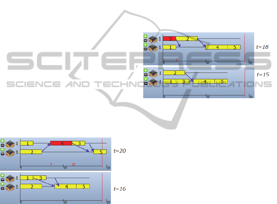
Figure 1 gives an example of delay reduction.

Task 3 does not depend on task 4, so moving task 4

to the first processor reduces the delay of task 3, and

the total time decreases accordingly.

Figure 1: Delay reduction strategy example.

Idle Time Reduction Strategy (strategy S2). This

strategy is based on the assumption that in the best

schedule the total time when the processors are idle

and no tasks are executed due to waiting for data

transfer to end is minimal.

For each position (m, n) the idle time is defined

as follows. If n=1 then its idle time is the time

between the beginning of the work and the start of

the execution of the task in the position (m, 1). If the

position (m, n) denotes the place after the end of the

last task on the processor m, then its idle time is the

time between the end of the execution of the last

task on m and the end of the whole program.

Otherwise, the idle time of the position (m, n) is the

interval between the end of the task in (m, n-1) and

the beginning of the task in (m, n).

The task to move is selected randomly with

higher probability assigned to the tasks executed

later. Among all positions where it is possible to

move the selected task, the position with the highest

idle time is selected. If the operation is not accepted,

the position with the second highest idle time is

selected, and so on.

The idle time reduction strategy is illustrated in

Figure 2. The idle time between tasks 1 and 4 is

large and thus moving task 3 allows reducing the

total execution time.

Figure 2: Idle time reduction strategy example.

Mixed Strategy (Strategy S3). As the name suggests,

the mixed strategy is a combination of the two

previous strategies. One of the two strategies is

selected randomly on each iteration. The aim of this

strategy is to find parts of the schedule where some

processor is idle for a long period and to try moving

a task with a big delay there, prioritizing earlier

positions to reduce the delay as much as possible.

This strategy has the benefits of both idle time

reduction and delay reduction, however, more

iterations may be required to reach the solution.

After performing the operation a new schedule is

created and time, reliability and number of

processors are calculated for it. Depending on the

values of these three functions the new schedule can

be accepted as the new approximation for the next

iteration of the algorithm. The probability to accept a

worse schedule on step 3 depends on the parameter

called temperature. This probability decreases along

with the temperature over time. Temperature

functions such as Boltzmann and Cauchy laws

(Wasserman, 1989) can be used as in most simulated

annealing algorithms.

The correctness of the algorithm can be inferred

from the fact that on all iterations the schedule is

modified only by operations introduced in this

section, and according to theorem 2, each operation

leads to a correct schedule.

ICORES2014-InternationalConferenceonOperationsResearchandEnterpriseSystems

Theorem 3 (Asymptotic Convergence). Assume that

the temperature values decrease at logarithmic rate

or slower: t



Г/logkk



,Г0,k



2.

Then the simulated annealing algorithm converges

in probability to the stationary distribution where the

probability to reach an optimal solution is q









i, where  is the set of optimal solutions.

Proof. As shown in (Lundy, 1986), the simulated

annealing algorithm can be represented with an

inhomogeneous Markov chain. The stationary

distribution exists if the Markov chain is strongly

ergodic. The necessary conditions of strong

ergodicity are (1) weak ergodicity, (2) the matrix







has an eigenvalue equal to 1 for each k, (3)

for its eigenvectors q(k) the series

∑‖



















1



‖



converges (Van Laarhoven, 1992). First

we need to prove that the Markov chain is strongly

ergodic. Condition (2) means that there exists an

eigenvector q such that P







⋅qq, or for each

row of the matrix, q





∑



⋅P

∈

, which is exactly

equivalent to the detailed balance equations. It is

possible to check that





|ε





∑



|

⋅

min1,e























min1,e



























Is the solution of this set of equations.

Let min1,e





















A



. Notice that the

following equation holds: A



⋅A



A



Now it is easy to check the detailed balance

equations.

|ε





∑



|

⋅











⋅A







|

∑





|

⋅











⋅A



∑



|

⋅











∑





|

⋅









⋅







∑



|

⋅











∑





|

⋅





⋅









∑



|

⋅











∑





|

⋅









The last equation is obviously correct.

To check condition (3) the following calculations

can be performed.



‖





q



k1

‖

















q





k1

|















|

∑





|

⋅





















|

∑





|

⋅





k1







k1

















C⋅



∑

A



k/A



k





∑

A



k1/A



k1













⋅



∑

A



1/A



1





∑

A



k/A



k







Considering the conditions of the theorem, the last

item is proportional to 1/k, and thus it converges to

To check condition (1) it is possible to use the

necessary condition of weak ergodicity (Van

Laarhoven, 1992): prove that the series

∑

1







P









 diverges. Let us find a lower bound for

P(k).





min

,



⋅exp

min1,f





f











C







/



1τ













C



















/







Considering that t















, we have a series

like C⋅

∑









, that diverges.

Finally it is necessary to find the limit of the

vector q when the temperature approaches 0. Let us

examine the limit of the expression in the

denominator.

lim

→



min1,e























min1,e



























If solution i is optimal, then the denominator is

always equal to 1 regardless of j. The numerator will

be equal to 1 is j is also an optimal solution, i.e.

f(i)=f(j), otherwise, if f(i)<f(j), then e





















→0. So,

the item in the sum converges to 1 if it corresponds

to an optimal solution j, and converges to 0

otherwise. Therefore the limit is



, and q









If solution i is not optimal, then in one of the

denominators contains f(j)-f(i)>0, and so the

sequence e





















→∞, and the corresponding



→0.

Finally we can conclude that q









i,

Q.E.D.

Theorem 5. The computational complexity of one

iteration is O(N(N+E)), where N is the number of

vertices of the program graph G and E is the number

of its edges (Zorin, 2012).

JobShopSchedulingandCo-DesignofReal-TimeSystemswithSimulatedAnnealing

4 EXPERIMENTS

The algorithm was tested both on artificial and

practical examples. Artificial tests are necessary to

examine the behavior of the algorithm on a wide

range of examples. As the general convergence is

theoretically proved, the aim of the experiments is to

find the actual speed of the algorithm and to

compare different strategies among each other.

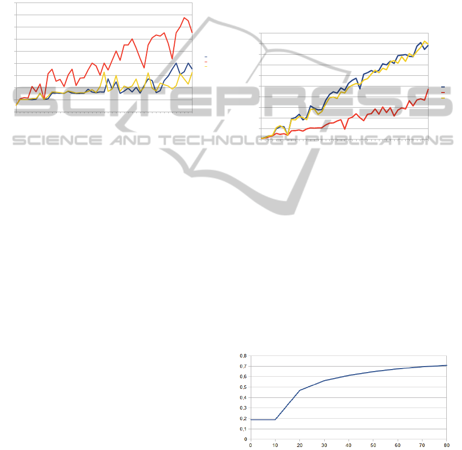
Figure 3: Comparison of the strategies.

Graph on figure 3 shows the results of the

comparison of three strategies. We generated

random program graphs with a pre-defined number

of vertices and the number of edges proportional to

the number of vertices. The number of vertices

varies from 5 to 225 with step 5. For each example

the algorithm was run 300 times, 100 times for each

strategy, to make the results statistically important.

The number of iterations of the algorithm was set

fixed.

Figure 3 shows the average value of the target

function (number of processors) depending on the

number of vertices. The functions are not

monotonous because of the random nature of the

examples: it is not possible to guarantee that a

solution with some number of processors exists, so a

program of n tasks might require more processors

than a program of n+5 tasks. The idle time reduction

strategy works worse than the other two, which is a

sharp contrast with the previous version of the

algorithm as shown in (Zorin, 2012).

The following statistical hypotheses (Sprinthall,

2006) hold for the conducted sample of experiments.

1. Strategy S2 gives worse results than S1 and S3

2. Strategy S3 gives a result that is worse by not

more than one processor, equal or better that the

result of S1.

3. The results given by the algorithm are locally

optimal.

Figure 4 shows the number of iterations required to

reach the best result found for the corresponding

problem. In each experiment, the algorithm

conducted 10N operations, where N is the number of

tasks, however, after some point the continuing

iteration stopped improving the result. Experiments

show that the speed of the mixed strategy is

practically equal to the speed of the delay reduction

strategy, with S3 being slightly faster. Idle time

reduction strategy is significantly faster, but it can be

explained with the low quality of its results, hence

fewer steps are needed to reach such results.

Figure 4: Comparison of the speed of the strategies.

The practical problem we solved with the

proposed algorithm is related to the design of

radiolocation systems and is described in detail in

(Kostenko, 1994) and (Zorin, 2013, SYRCoSE).

Briefly, the problem is to find the minimal number

of processors needed to conduct the computation of

the source of radio signals. The signals are received

by an antenna array and then a special parallel

method is used computes the results. The method is

based on splitting the whole frequency diapason into

L intervals and calculating the data for each interval

separately, preferably on parallel processors. Each of

L threads is split into M subthreads as well.

Figure 5: Optimization rate (X axis shows the values of L,

Y axis shows the optimization rate).

In real systems the size of the array is a power of

2, usually between 256 and 1024 and the number of

100

105

110

115

120

125

130

135

140

145

150

155

160

165

170

175

180

185

190

195

200

205

210

215

220

225

Num ber of tas ks

Number of processors

100

105

110

115

120

125

130

135

140

145

150

155

160

165

170

175

180

185

190

195

200

205

210

215

220

225

100

200

300

400

500

600

700

800

900

1000

Number of tasks

Number of iterations

ICORES2014-InternationalConferenceonOperationsResearchandEnterpriseSystems

frequency intervals (L) is also power of 2, usually 32

or 64. M is a small number, usually between 2 and 5.

As the vast majority of complex computations are

done after splitting to frequency intervals, L is the

main characteristic of the system that influences the

overall performance. Therefore, the quality of the

algorithm can be estimated by comparing the

number of processors in the result with the default

system configuration where L*M processors are

used. Figure 5 shows the quotient of these two

numbers, depending on L, for radiolocation problem.

Lower quotient means better result of the algorithm.

As we can see, the algorithm optimizes the

multiprocessor system by at least 25% in harder

examples with many parallel tasks, and by more than

a half in simpler cases.

5 CONCLUSIONS

In this paper we formulate a combinatorial

optimization problem arising from the problem of

co-design of real-time systems. We suggest a

heuristic algorithm based on simulated annealing,

provide its description and prove the basic features,

including asymptotic convergence.

Experimental evaluation of the different

heuristic strategies within the discussed algorithm

showed that one of the strategies was lacking

compared to the other two. Mixed and delay

reduction strategies have equal quality, while the

mixed strategy converges slightly faster.

REFERENCES

Antonenko V. A., E. V. Chemeritsky, A. B. Glonina, I. V.

Konnov, V. N. Pashkov, V. V. Podymov, K. O.

Savenkov, R. L. Smelyansky, P. M. Vdovin, D. Yu.

Volkanov, V. A. Zakharov, D. A. Zorin (2013)

DYANA: an integrated development environment for

simulation and verification of real-time avionics

systems. Munich: European Conference for

Aeronautics and Space Sciences (EUCASS).

Avizienis, A., Laprie, J.C. and Randell, B. (2004).

Dependability and its threats: a taxonomy. Toulouse:

Building the Information Society Proc IFIP 18th

World Computer Congress, 91-120.

Balashov V. V., Balakhanov V. A., Kostenko V. A.,

Smelyansky R. L., Kokarev V. A., Shestov P. E.

(2010) A technology for scheduling of data exchange

over bus with centralized control in onboard avionics

systems. Proc. Institute of Mechanical Engineering,

Part G: Journal of Aerospace Engineering, 224, No. 9,

993–1004.

Eckhardt, D. E. and Lee, L.D. (1985). A theoretical basis

for the analysis of multiversion software subject to

coincident errors. IEEE Transactions on Software

Engineering, 11, 1511-1517.

Goldberg, D. E. (1989). Genetic algorithms in search,

optimization, and machine learning. Addison Wesley.

Hou, E. S., Hong, R., & Ansari, N. (1990, November).

Efficient multiprocessor scheduling based on genetic

algorithms. In Industrial Electronics Society, 1990.

IECON'90., 16th Annual Conference of IEEE (pp.

1239-1243). IEEE.

Jedrzejowicz, P., Czarnowski, I., Szreder, H., &

Skakowski, A. (1999). Evolution-based scheduling of

fault-tolerant programs on multiple processors. In

Parallel and Distributed Processing (pp. 210-219).

Springer Berlin Heidelberg.

Laprie J.-C., Arlat J., Beounes C. and Kanoun K. (1990).

Definition and analysis of hardware- and software-

fault-tolerant architectures. Computer, 23, 39-51.

Kalashnikov, A. V. and Kostenko, V. A. (2008). A

Parallel Algorithm of Simulated Annealing for

Multiprocessor Scheduling. Journal of Computer and

Systems Sciences International, 47, No. 3, 455-463.

Kirkpatrick, S., Jr., D. G., & Vecchi, M. P. (1983).

Optimization by simulated annealing. Science,

220(4598), 671-680.

Kostenko, V. A. (1994). Design of computer systems for

digital signal processing based on the concept of

“open” architecture. Avtomatika i Telemekhanika,

(12), 151-162.

Kostenko V. A., Romanov V. G., Smelyansky R. L.

(2000). Algorithms of minimization of hardware

resources. Artificial Intelligence, 2, 383-388

Kostenko V. A. (2002). The Problem of Schedule

Construction in the Joint Design of Hardware and

Software. Programming and Computer Software, 28,

No. 3, 162–173.

Lundy, M., & Mees, A. (1986). Convergence of an

annealing algorithm. Mathematical programming,

34(1), 111-124.

Moore, M. (2003). An accurate and efficient parallel

genetic algorithm to schedule tasks on a cluster. In

Parallel and Distributed Processing Symposium,

2003. Proceedings. International (pp. 5-pp). IEEE.

Orsila, H., Salminen, E., & Hämäläinen, T. D. (2008).

Best practices for simulated annealing in

multiprocessor task distribution problems. Simulated

Annealing, 321-342.

Qin, X., Jiang, H., & Swanson, D. R. (2002). An efficient

fault-tolerant scheduling algorithm for real-time tasks

with precedence constraints in heterogeneous systems.

In Parallel Processing, 2002. Proceedings.

International Conference on(pp. 360-368). IEEE.

Qin, X., & Jiang, H. (2005). A dynamic and reliability-

driven scheduling algorithm for parallel real-time jobs

executing on heterogeneous clusters. Journal of

Parallel and Distributed Computing, 65(8), 885-900.

Smelyansky R. L., Bakhmurov A. G., Volkanov D. Yu.,

Chemeritskii E. V. (2013) Integrated Environment for

the Analysis and Design of Distributed Real-Time

JobShopSchedulingandCo-DesignofReal-TimeSystemswithSimulatedAnnealing

Embedded Computing Systems. Programming and

Computer Software, 39, No. 5, 242-254

Sprinthall, R. C. (2006). Basic Statistical Analysis. Allyn

& Bacon

Van Laarhoven, P. J., Aarts, E. H., & Lenstra, J. K.

(1992). Job shop scheduling by simulated annealing.

Operations research, 40(1), 113-125.

Wasserman, P. D. (1989). Neural computing: theory and

practice. Van Nostrand Reinhold Co..

Wattanapongsakorn, N. and Levitan, S.P. (2004).

Reliability optimization models for embedded systems

with multiple applications. IEEE Transactions on

Reliability, 53, 406-416.

Zorin D.A. (2012) Comparison of different operation

application strategies in simulated annealing algorithm

for scheduling on multiprocessors. Moscow: Parallel

Computing (PACO-2012), V.1, 278-291

Zorin D.A. (2013) Scheduling Signal Processing Tasks for

Antenna Arrays with Simulated Annealing. Kazan:

Proceedings of the 7th Spring/Summer Young

Researchers’ Colloquium on Software Engineering

(SYRCoSE), 122-127.

ICORES2014-InternationalConferenceonOperationsResearchandEnterpriseSystems