Unsupervised Consensus Functions Applied to Ensemble Biclustering

Blaise Hanczar and Mohamed Nadif

LIPADE, University Paris Descartes, 45 rue des saint-peres, 75006 Paris, France

Keywords:

Biclustering, Ensemble Methods, Consensus Functions.

Abstract:

The ensemble methods are very popular and can improve signiﬁcantly the performance of classiﬁcation and

clustering algorithms. Their principle is to generate a set of different models, then aggregate them into only

one. Recent works have shown that this approach can also be useful in biclustering problems.The crucial

step of this approach is the consensus functions that compute the aggregation of the biclusters. We identify

the main consensus functions commonly used in the clustering ensemble and show how to extend them in

the biclustering context. We evaluate and analyze the performances of these consensus functions on several

experiments based on both artiﬁcial and real data.

1 INTRODUCTION

Biclustering, also called direct clustering (Hartigan,

1972), simultaneous clustering in (Govaert, 1995;

Turner et al., 2005) or block clustering in (Govaert

and Nadif, 2003) is now a widely used method of data

mining in various domains in particular in text mining

and bioinformatics. For instance, in document clus-

tering, in (Dhillon, 2001) the author proposed a spec-

tral block clustering method which makes use of the

clear duality between rows (documents) and columns

(words). In the analysis of microarray data, where

data are often presented as matrices of expression lev-

els of genes under different conditions, the co- clus-

tering of genes and conditions overcomes the problem

encountered in conventional clustering methods con-

cerning the choice of similarity. Cheng and Church

(Cheng and Church, 2000) were the ﬁrst to propose

a biclustering algorithm for microarray data analy-

sis. They considered that biclusters follow an addi-

tive model and used a greedy iterative search to mini-

mize the mean square residue (MSR). Their algorithm

identiﬁes the biclusters one by one and was applied to

yeast cell cycle data, and made it possible to identify

several biologically relevant biclusters. Lazzeroni and

Owen (Lazzeroni and Owen, 2000) have proposed

the popular plaid model which has been improved by

Turner et al. (Turner et al., 2005). The authors as-

sumed that biclusters are organized in layers and fol-

low a given statistical model incorporating additive

two way ANOVA models. The search approach is it-

erative: once (K − 1) layers (biclusters) were identi-

ﬁed, the K-th bicluster minimizing a merit function

depending on all layers is selected. Applied to data

from the yeast, the proposed algorithm reveals that

genes in biclusters share the same biological func-

tions. In (Erten and S

ozdinler, 2010) the authors de-

veloped their localization procedure which improves

the performance of a greedy iterative biclustering al-

gorithm. Several other methods have been proposed

in the literature, two complete surveys of biclustering

methods can be found in (Madeira and Oliveira, 2004;

Busygin et al., 2008).

Here we propose to use the ensemble methods to

improve the performance of biclustering. It is impor-

tant to note that we do not propose a new biclustering

method in competition with the previously mentioned

algorithms. We seek to adapt the ensemble approach

to the biclustering problem in order to improve the

performance of any biclustering algorithm. The prin-

ciple of ensemble biclustering is to generate a set of

different biclustering solutions, then aggregate them

into only one solution. The crucial step is based on

the consensus functions computing the aggregation of

the different solutions. In this paper we have identi-

ﬁed four types of consensus function commonly used

in ensemble clustering and giving the best results. We

show how to extend their use in the biclustering con-

text. We evaluate their performances on a set of both

numerical and real data experiments.

The paper is organized as follows. In Section 2,

we review the ensemble methods in clustering and bi-

clustering. In section 3, we formalize the collection

of biclustering solutions and show how to construct

it from the Cheng & Church algorithm that we chose

for our study. In section 4, we extend four commonly

Hanczar B. and Nadif M..

Unsupervised Consensus Functions Applied to Ensemble Biclustering.

DOI: 10.5220/0004789800300039

In Proceedings of the 3rd International Conference on Pattern Recognition Applications and Methods (ICPRAM-2014), pages 30-39

ISBN: 978-989-758-018-5

 2014 SCITEPRESS (Science and Technology Publications, Lda.)

used consensus functions to the biclustering context.

Section 5 is devoted to evaluate these new consen-

sus functions on several experimentations. Finally,

we summarize the main points resulting from our ap-

proach.

2 ENSEMBLE METHODS

The principle of ensemble methods is to construct a

set of models, then to aggregate them into a single

model. It is well-known that these methods often per-

form better than a single model (Dietterich, 2000).

Ensemble methods ﬁrst appeared in supervised learn-

ing problems. A combination of classiﬁers is more

accurate than single classiﬁers (Maclin, 1997). A pi-

oneer method boosting, the most popular algorithm

which is adaboost, was developed mainly by Shapire

(Schapire, 2003). The principle is to assign a weight

to each training example, then several classiﬁers are

learned iteratively and between each learning step the

weight of the examples is adjusted depending on the

classiﬁer results. The ﬁnal classiﬁer is a weighted

vote of classiﬁers constructed during the procedure.

Another type of popular ensemble methods is bag-

ging, proposed by Breiman (Breiman, 1996). The

principle is to create a set a classiﬁers based on boot-

strap samples of the original data. The random forests

(Breiman, 2001) are the most famous application of

bagging. They are a combination of tree predictors,

and have given very good results in many domains

(Diaz-Uriarte and Alvarez de Andres, 2006).

Several works have shown that ensemble methods

can also be used in unsupervised learning. Topchy et

al. (Topchy et al., 2004b) showed theoretically that

ensemble methods may improve the clustering per-

formance. The principle of boosting was exploited

by Frossyniotis et al. (Frossyniotis et al., 2004) in

order to provide a consistent partitioning of the data.

The boost-clustering approach creates, at each itera-

tion, a new training set using weighted random sam-

pling from original data, and a simple clustering algo-

rithm is applied to provide new clusters. Dudoit and

Fridlyand (Dudoit and Fridlyand, 2003) used bagging

to improve the accuracy of clustering in reducing the

variability of the PAM algorithm (Partitioning Around

Medoids) results (van der Laan et al., 2003). Their

method has been applied to leukemia and melanoma

datasets and made it possible to differentiate the dif-

ferent subtypes of tissues. Strehl et al. (Strehl and

Ghosh, 2002) proposed an approach to combine mul-

tiple partitioning obtained from different sources into

a single one. They introduced heuristics based on a

voting consensus. Each example is assigned to one

cluster for each partition, an example has therefore as

many assignments as number of partitions in the col-

lection. In the aggregated partition, the example is

assigned to the cluster to which it was the most of-

ten assigned. One problem with this consensus is that

it requires knowledge of the cluster correspondence

between the different partitions. They also proposed

a cluster-based similarity partitioning algorithm. The

collection is used to compute a similarity matrix of

the examples. The similarity between two examples

is based on the frequency of their co-association to

the same cluster over the collection. The aggregated

partition is computed by a clustering of the exam-

ples from the similarity matrix. Fern (Fern and Brod-

ley, 2004) formalized the aggregation procedure by a

bipartite graph partitioning. The collection is repre-

sented by a bipartite graph. The examples and clus-

ters of partitions are the two sets of vertices. An edge

between an example and a cluster means that exam-

ple has been assigned to this cluster. A partition of

the graph is performed and each sub-graph represents

an aggregated cluster. Topchy (Topchy et al., 2004a)

proposed to modelize the consensus of the collection

by a multinomial mixture model. In the collection,

each example is deﬁned by a set of labels that rep-

resents their assigned clusters in each partition. This

can be seen as a new space in which the examples are

deﬁned, each dimension being a partition of the col-

lection. The aggregated partition is computed from a

clustering of examples in this new space. Since the

labels are discrete variables, a multinomial mixture

model is used. Each component of the model repre-

sents an aggregated cluster.

Some recent works have shown that the ensem-

ble approach can also be useful in biclustering prob-

lems (Hanczar and Nadif, 2012). DeSmet pre-

sented a method of ensemble biclustering for query-

ing gene expression compendia from experimental

lists (De Smet and Marchal, 2011). Actually the en-

semble approach is performed only one dimension of

the data (the gene dimension). Then biclusters are ex-

tracted from the gene consensus clusters. A bagging

version of biclustering algorithms has been proposed

and tested for microarray data (Hanczar and Nadif,

2010). Although this last method improves the per-

formance of biclustering, in some cases it fails and

returns empty biclusters, i.e. without examples or fea-

tures. This is because the consensus function handles

the sets of examples and features on the same dimen-

sion as in the clustering context. The consensus func-

tion must respect the structure of the biclusters. For

this reason, the consensus functions mentioned above,

can be applied to biclustering problems. In this paper

we adapt these consensus functions to the biclustering

UnsupervisedConsensusFunctionsAppliedtoEnsembleBiclustering

context.

3 BICLUSTERING SOLUTION

COLLECTION

The ﬁrst step of ensemble biclustering is to generate

a collection of biclustering solution. Here we give

the formalization of the collection and a method to

generate it from the Cheng and Church algorithm that

we have chosen for our study.

3.1 Formalization of the Collection

Let a data matrix be = { , } where =

,...,e

} is the set of N examples represented by

M-dimensional vectors and = { f

,..., f

} is the

set of M features represented by N-dimensional vec-

tors. A bicluster B is a submatrix of X deﬁned

by a subset of examples and a subset of features:

B = {(E

)|E

⊆ ,F

⊆ }. A biclustering op-

erator Φ is a function that returns a biclustering so-

lution (i.e. a set of biclusters) from a data matrix:

Φ(X) = {B

,...,B

} where K is the number of bi-

clusters. Let ϕ be the function giving for each point

of the data matrix the label of the bicluster to which

it belongs. The label is 0 for points belonging to no

bicluster.

ϕ(x

i j

) =

{

k i f e

∈ E

and f

∈ F

0 i f e

/∈ E

or f

/∈ F

∀k ∈ [1,K].

A biclustering solution can be represented by a label

matrix I

giving for each point: I

i j

= ϕ(x

i j

). In the

following it will be convenient to represent this label

matrix by an label vector indexed by u deﬁned as u =

i ∗| | +(| | − j), where |.| denotes the cardinality. J

is the vector form of the matrix I

: J

= J

i∗| |+(| |− j

ϕ(x

i j

Let’s the true biclustering solution of the data set

represented by Φ( )

∗

, I

∗

and J

∗

. An estimated bi-

clustering solution is a biclustering solution returned

by an algorithm from the data matrix, it is denoted by

Φ( ),

and

. The objective of the biclustering task is

to ﬁnd the closest estimated biclustering solution from

the true biclustering solution. In ensemble methods,

we do not use only one estimated biclustering solu-

tions but we generate a collection of several solutions.

We denote this collection of biclustering solutions

as follows = {

Φ(X)

(1)

,...,

Φ(X)

(R)

}. This collec-

tion can be represented by an NM × R matrix =

,...,J

)

by merging together all label vectors

= (J

,...,J

)

where J

= ϕ(x

i j

)

(r)

with r ∈

[1,R]. The objective of the consensus function is to

form an aggregated biclustering solution, represented

by Φ(X), I

and J

, from the collection of estimated so-

lutions. Each of these functions is illustrated with an

example in Figure 1.

3.2 Construction of the Collection

The key point of the generation of the collection is

to ﬁnd a good trade-off between the quality and di-

versity of the biclustering solutions of the collection.

If all the generated solutions are the same, the aggre-

gated solution is identical to the biclusters of the col-

lection. Different sources of the diversity are possible.

We can use a resampling method such as bootstrap

or jacknife. In applying the biclustering operator to

each resampled data, different solutions are produced.

We can also include the source of diversity directly in

the biclustering operator. In this case the algorithm is

not deterministic and will produce different solutions

from the same original data.

In our experiments the biclustering operator is the

Cheng and Church algorithm (CC) (algorithm 4 in the

reference (Cheng and Church, 2000)). This algorithm

returns a set of biclusters minimizing the mean square

residue ( MSR).

MSR(B

) =

∑

i, j

i j

− µ

+ µ

)

where µ

is the average of B

, µ

and µ

are respec-

tively the means of E

and F

belonging to bicluster

. z and w are the indicator functions of the exam-

ples and features. z

= 1 when the feature i belongs

to the bicluster k, z

= 0 otherwise. w

= 1 when the

example j belongs to the bicluster k, w

= 0 other-

wise.

The CC algorithm is iterative and the biclusters

are identiﬁed one by one. To detect each bicluster, the

algorithm begins with all the features and examples,

then it drops the feature or example minimizing the

mean square residue (MSR) of the remaining matrix.

This procedure is totally deterministic. We modiﬁed

the CC algorithm by including a source of diversity in

the computation of the bicluster. At each iteration, we

selected the top α% of the features and examples min-

imizing MSR of the remaining matrix. The element to

be dropped was randomly chosen from this selection.

Thus the parameter α controls the level of diversity

of the bicluster collection; in our simulations α = 5%

seemed a good threshold. This modiﬁed version of

the algorithm was used in all our experiments in or-

der to generate the collection of biclustering solutions

from a dataset.

ICPRAM2014-InternationalConferenceonPatternRecognitionApplicationsandMethods

4 CONSENSUS FUNCTIONS FOR

BICLUSTERING

The second step of the ensemble approach is the ag-

gregation of the collection of biclustering solutions.

We present here the extension of four consensus func-

tions for biclustering ensemble. These methods as-

sign a bicluster label to the N × M points of the data

matrix. Note that even when the numbers of biclus-

ters in the different solutions of the collection are not

equal, these consensus functions can be used; it suf-

ﬁces to ﬁx the ﬁnal number of aggregated biclusters

to K.

4.1 CO-Association Consensus (COAS)

The idea of COAS is to group in a bicluster the points

that are assigned together in the biclustering collec-

tion. This consensus is based on the bicluster assig-

nation similarity between the points of the data ma-

trix. The similarity between two points is deﬁned by

the proportion of times that they are associated to the

same bicluster over the whole collection. All these

similarities are represented by a distance matrix D de-

ﬁned by:

= 1 −

∑

r=1

δ(J

= J

where δ(x) returns 0 when x is false and 1 when true.

From this dissimilarity data matrix, K + 1 clusters are

identiﬁed in using the Partitioning Around Medoids

(PAM) algorithm (Dudoit and Fridlyand, 2003). The

K clusters of points represent the K aggregated biclus-

ters, the last cluster groups all the points that belongs

to no bicluster.

4.2 Voting Consensus (VOTE)

This consensus function is based on the majority vote

of the labels. Each point is assigned to the bicluster

with which it has been assigned the most of the time in

the biclustering collection. For each point of the data

matrix, the consensus returns the most represented la-

bel in the collection of the biclustering solution. The

main problem of this approach is that there is no cor-

respondence between the labels of two different esti-

mated biclustering solutions. All the biclusters of the

collection have to be re-labeled according to their best

agreement with some chosen reference solution. Any

estimated solution can be used as reference, here we

used the ﬁrst one

Φ(X)

(1)

. The agreement problem

can be solved in polynomial time by the Hungarian

method (Papadimitriou and Steiglitz, 1982) which re-

labels the estimated solution such the similarity be-

tween the solutions is maximized. The similarity be-

tween two biclustering solutions was computed by us-

ing the F-measure (details in section 5.1). The label

of the aggregated biclustering solution for a point is

therefore deﬁned by:

= argmax

(

∑

r=1

δ(Γ(J

) = k)

)

where Γ is the relabelling operator performed by the

Hungarian algorithm.

4.3 Bipartite Graph Partitionning

Consensus (BGP)

In this consensus the collection of estimated solutions

is represented by a bipartite graph where the vertices

are divided into two sets: the point vertices and the

label vertices. The point vertices represent the points

of the data matrix {(e

, f

)} while the set of label ver-

tices represents all the estimated biclusters of the col-

lection {

k,(r)

}, for each estimated solution there is

also a vertice that represents the points belonging to

no bicluster. An edge links a point vertice to a label

vertice if the point belongs to the corresponding esti-

mated bicluster. The degree of each point is therefore

R and the degree of each estimated bicluster repre-

sents the number of points that it contains. Finding

a consensus consists in ﬁnding a partition of this bi-

partite graph. The optimal partition is the one that

maximizes the numbers of edges inside each cluster

of nodes and minimizes the number of edges between

nodes of different clusters. This graph partitioning

problem is a NP-hard problem, so we rely on a heuris-

tic to an approximation of the optimal solution. We

used a method based on a spin-glass model and sim-

ulated annealing (Reichardt and Bornholdt, 2006) in

order to identify the clusters of nodes. Each clus-

ter of the partition represents an aggregated bicluster

formed by all the points contained in this cluster.

4.4 Multivariate Mixture Model

Consensus (MIX)

In (Topchy et al., 2004a), the authors have used the

mixture approach to propose a consensus function. In

the sequel we propose to extend it to our situation.

In model-based clustering it is assumed that the data

are generated by a mixture of underlying probability

distributions, where each component k of the mixture

represents a cluster. Speciﬁcally, the NM × R data

matrix is assumed to be an J

,...,J

i.i.d

UnsupervisedConsensusFunctionsAppliedtoEnsembleBiclustering

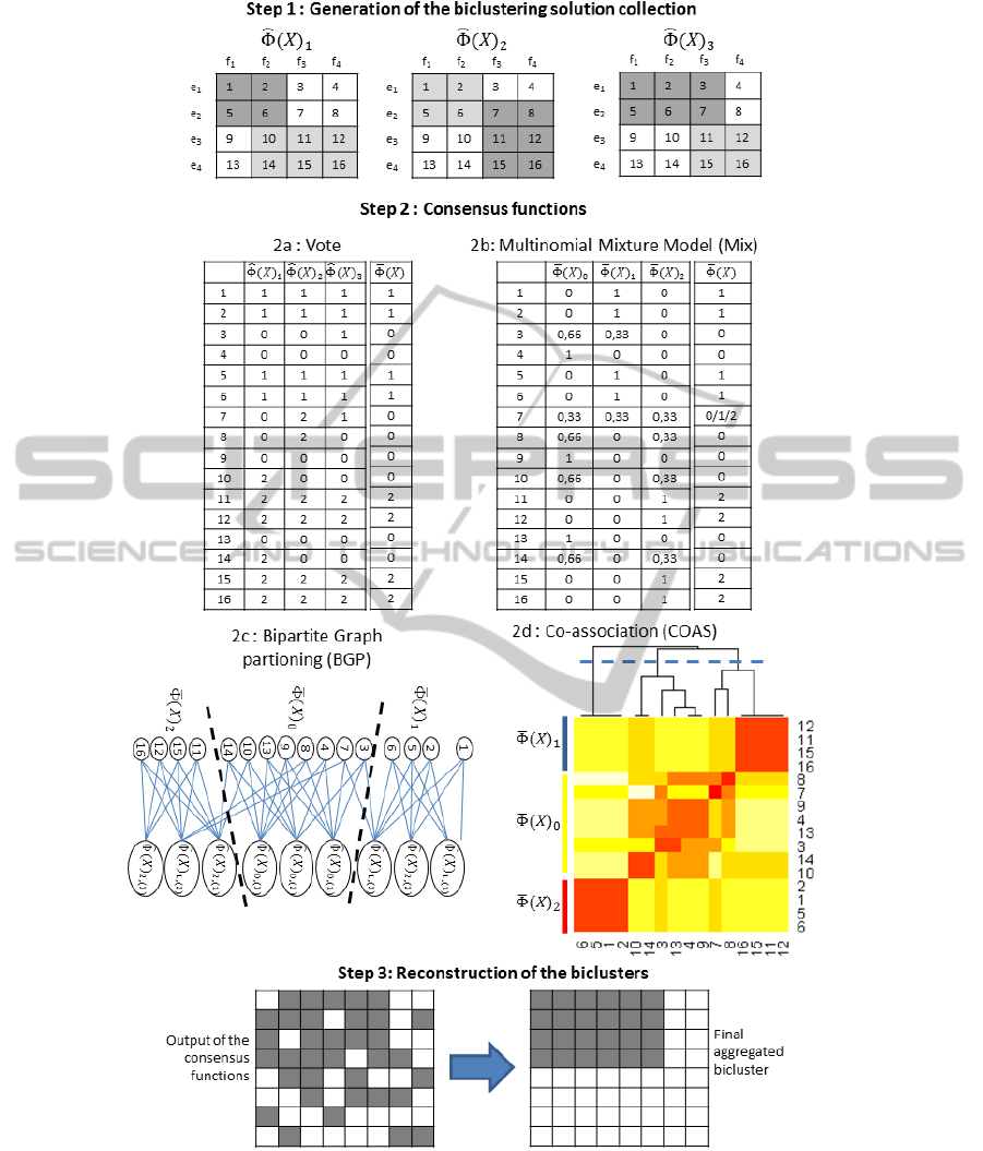
Figure 1: Procedure of ensemble biclustering with the four consensus functions. 1) 3 different biclustering solutions with 2

biclusters for the same data matrix forming the collection. 2a) The collumns represents the labels of each data points obtained

by the three biclustering solution. The last column represents the results of the VOTE consensus. 2b) The ﬁrst three columns

give the probability for each data point to be associated to the three labels of the mixture model. The last column represents

the results of the MIX consensus. 2c) The bipartite graph representing all biclusters of the collection. The cuts of the graph

give the results of the BGP consensus. 2d) The coassociation matrice of the data points. The 3 clusters obtained from this

matrix represent the results of the COAS consensus. 3) An example of the reconstruction step of our methods.

ICPRAM2014-InternationalConferenceonPatternRecognitionApplicationsandMethods

sample where J

from a probability distribution with

density

φ(J

|Θ) =

∑

k=0

|θ

where P

|θ

) is the density of label J

from the kth

component and the θ

s are the corresponding class

parameters. These densities belong to the same para-

metric family. The parameter π

is the probability that

an object belongs to the kth component, and K, which

is assumed to be known, is the number of components

in the mixture. The number of components corre-

sponds to the number of biclusters minus one since

one of the components represents the points belong-

ing to no bicluster. The parameter of this model is

the vector Θ = (p

,...,p

,θ

,...,θ

). The mixture

density of the observed data can be expressed as

φ( |Θ) =

∏

u=1

∑

k=0

|θ

The J

labels are nominal categorical variables, we

consider the latent class model and assume that all R

categorical variables are independent, conditionnally

on their memebership of a component;

|θ

) =

∏

r=1

k,(r)

|θ

k,(r)

Note that P

k,(r)

|θ

k,(r)

) represents the probability to

have J

labels in the kth component for the estimated

solution

Φ(X)

(r)

. If α

r( j)

is the probability that the

rth label takes the value j when an J

belongs to the

component k, then the probability of the mixture can

be written P

|θ

) =

∏

r=1

∏

j=1

[α

r( j)

]

δ(J

= j)

. The

parameter of the mixture Θ is ﬁtted in maximizing

the likelihood function:

∗

= argmax

(

log

(

∏

u=1

P(J

|θ)

))

The optimal solution of this maximization problem

cannot generally be computed, we therefore rely on

an estimation given by the EM algorithm (Dempster

et al., 1977). In E-step, we compute the posterior

probabilities of each label s

∝ P

|θ

) and in the

M-step we estimate the parameters of the mixture as

follows

∑

and α

r( j)

∑

δ(J

= j)

∑

To limit the problems of local minimum during the

EM algorithm, we performd the optimization process

ten times with different initializations and kept the so-

lution maximizing the log-likelihood. At the conver-

gence, we consider that the largest π

corresponds to

S1 S2 S3 S4

Figure 2: The four data structures considered in the experi-

ments.

labels representing the points belonging to no biclus-

ters. The estimators of posterior probabilities give

rise to a fuzzy or hard clustering using the maxi-

mum a posteriori principle (MAP). Then the consen-

sus function consists in taking for each J

the clus-

ter such that k maximizing its conditional probability

k = argmax

ℓ=1,...,K

uℓ

, and we obtained the ensemble

solution noted Φ( ).

4.5 Reconstruction of the Biclusters

The four consensus functions presented above, return

a partition in K + 1 clusters of the points of the data

matrix. K of these clusters represent the K aggregated

biclusters, the last one groups all the points that be-

long to no biclusters in the aggregated solution. The

k aggregated biclusters are not actual biclusters yet.

They are just sets of points that do not necessarily

form submatrices of the data matrix. A reconstruction

step has to be applied to each aggregated bicluster in

order to transform it into a submatrix. This proce-

dure consists in ﬁnding the submatrix containing the

maximum of points that are in the aggregated biclus-

ter and the minimum of points that are not in the ag-

gregated bicluster. The k-th aggregated bicluster is

reconstructed by minimizing the following function:

L(B

) =

∑

i=1

∑

j=1

δ(e

∈ E

∧ f

∈ F

)δ(I

i j

̸= k)

+ δ(e

/∈ E

∨ f

/∈ F

)δ(I

i j

= k).

This optimization problem is solved by a heuristic

procedure. We started with all the examples and fea-

tures involved in the aggregated bicluster. Then iter-

atively, we dropped the example or feature that max-

imizes the decrease of L(B

). This step was iterated

until L(B

) did not decrease. Once the reconstruction

procedure was ﬁnished, we obtained the ﬁnal aggre-

gated biclusters.

UnsupervisedConsensusFunctionsAppliedtoEnsembleBiclustering

5 RESULTS AND DISCUSSION

5.1 Performance of Consensus

Functions

In our simulations, we considered four different data

structures with M = N = 100 in which a true bi-

clustering solution is included. The number of bi-

clusters varies from 2 to 6 and their sizes from 10

examples by 10 features to 30 examples by 30 fea-

tures. We have deﬁned four different structures of

biclusters depicted in Figure 2. For each data, from

each true bicluster an estimated bicluster was gener-

ated, then a collection of estimated biclustering so-

lutions was obtained. The quality of the collection

is controlled by the parameters α

pre

and α

rec

that

are the average precision and recall between esti-

mated biclusters and their corresponding true biclus-

ters. To generate an estimated bicluster we started

with the true bicluster, then we randomly removed

features/examples and have added features/examples

that were not in the true bicluster in order to ob-

tain the target precision α

pre

and recall α

rec

. Once

the collection was generated, the four consensus

functions were applied to obtain the aggregated bi-

clustering solutions. Finally to evaluate the perfor-

mance of each aggregated solution we computed the

average F-measure (noted ∆) between the obtained

solution Φ( ) and the true biclustering solution

Φ( )

∗

; ∆(Φ( )

∗

,Φ( )) =

∑

k=1

Fmes

∗

)

where M

Fmes

∗

) =

∗

∩B

∗

|+|B

is the F-measure.

Figure 3 shows the performance of the different

consensus in function on the size of the biclustering

solution collection R with α

pre

= α

rec

= 0.5. Each of

the six panels gives the results on the six data struc-

tures. The dot, triangle, cross and diamond curves

represent respectively the F-measure in function of R

for VOTE, COAS, BGP and MIX consensus. The full

gray curve represents the mean of the performance of

the biclustering collection. In the six panels, the per-

formance of the collection is constantly around 0.5.

That is be expected, since the performance of the col-

lection does not depend on its size and by construction

the theoretical performance of each estimated solu-

tion is 0.5. On the six dataset structures, from R ≥ 40,

all the consensus functions give much better perfor-

mances than the estimated solutions of the collec-

tion. The performances of MIX in all the situations

are strongly increasing with the size of the collection.

Mix does not require a high value of R to record good

results, for R ≥ 20 it converges to their maximum and

reaches 1 in all panels. The curves of BGP have the

same shape, they begin with a strong increase then

they converge to their maximums, but the increase

phase is much longer than in MIX. It also worth not-

ing that BGP begins with very low performances for

small values of R, it is often lower than the perfor-

mances of the collection. BGP reaches its best per-

formances with R ≥ 60, in four panels it obtains the

second best results and the third on the two last pan-

els. The performance of VOTE increases slowly and

more or less linearly with the collection size. Even

with very low values of R, the performance of the

consensus is signiﬁcantly better than the collection.

VOTE gives the second best performances for S1 and

S5 and the third best for the four other data structures.

The performance of COAS is more or less constant

whatever R; it obtains the worst results in all panels.

Figure 4 shows the performances of the different con-

sensus in function of the performances of the esti-

mated solution collection controlled by the parame-

ter α = α

pre

= α

rec

. The performances of all con-

sensus are naturally decreasing with α. By deﬁni-

tion the performances of the collection follow the line

y = 1 − x . For α ≤ 0.4 and in all the cases the con-

sensus functions give the almost perfect biclustering

solution with ∆ ≈ 1, expected for COAS in S4. MIX

is still clearly the best consensus, it produces almost

the perfect biclustering and its performances are never

less than 0.9. BGP is the second best consensus, it is

always signiﬁcantly better than the collection what-

ever the value of α. VOTE and COAS have simi-

lar behavior. They begin with the perfect bicluster-

ing solution then, when α ≥ 0.5, their performances

decrease and are at best, for VOTE, around the collec-

tion performance.

The F-measure can be decomposed into a combi-

nation of precision and recall. When we examine the

results in detail we see that for VOTE and COAS the

precision is much greater than the recall. That means

these consensus produce smaller biclusters than the

true ones, the features and examples associated to bi-

clusters are generally good but these biclusters are

incomplete i.e. examples and features are missing.

Conversely BGP produces biclusters with high re-

call and low precision. The aggregated biclusters are

generally complete but they also contain some extra

wrong features and examples. MIX gives balanced

biclusters with equal precision and recall. The exper-

iment on S4 makes it possible to observe the inﬂuence

of the size of the biclusters on the results. We can see

that COAS obtains very bad performance on the small

biclusters, since the recall on the two smallest biclus-

ters is 0. MIX, VOTE, COAS are independent from

the size of the biclusters, their performances are sim-

ilar with the four biclusters.

ICPRAM2014-InternationalConferenceonPatternRecognitionApplicationsandMethods

S1 S2 S3 S4

◦ : VOTE, △ : COAS, + : BGP, ♢ : MIX.

Figure 3: Performance of the consensus in function of R (size of the biclustering solution collection) with α

pre

= α

rec

= 0.5.

S1 S2 S3 S4

◦ : VOTE, △ : COAS, + : BGP, ♢ : MIX.

Figure 4: Performance of the consensus in function on the mean precision α

pre

and recall α

rec

of the biclustering solution

collection with α = α

pre

= α

rec

5.2 Results on Real Data

To evaluate our approach in terms of performance

on real datasets, we used four datasets: Nutt dataset

(gene expression), Pomeroy dataset (gene expres-

sion), Sonar dataset (Sonar signal) and Wdbc dataset

(biological dataset). Unlike numerical experiments

and since we do not known the true biclustering so-

lutions, the measures of performance can be based on

external indices, like Dice score. Obviously, the qual-

ity of a biclustering solution can be measured by the

AMSR i.e. the average of MSR computed from each

bicluster belonging to the biclustering solution; the

lower the AMSR, the better the solution. A problem

with this approach is that the MSR is biased by the

size of the biclusters. Indeed, the smallest biclusters

favour AMSR. To remove this size bias we set the size

of the biclusters in the parameters of the algorithms.

All the methods will therefore return biclusters of the

same size. The better solutions will be those mini-

mizing AMSR. To compare the different consensus

functions, we computed their gain which is the per-

centage of AMSR decreasing from the single biclus-

tering solution i.e. the solution obtained by the classic

CC algorithm without the ensemble approach. This is

computed by:

Gain = 100

AMSR(Φ

single

) − AMSR(Φ

ensemble

)

AMSR(Φ

single

)

where Φ

single

and Φ

ensemble

are the biclustering solu-

tion returned respectively by the single and ensemble

approaches.

Table 1 gives the gain of each consensus function

for all the datasets in function on the size of the bi-

clusters. We can observe that in all the situations, all

the consencus functions give an interesting gain, ex-

pected for COAS for Wdbc dataset. We know that in

the merging process, once a cluster is formed it does

not undo what was previously done; no modiﬁcations

or permutations of objects are therefore possible. This

disadvantage can be a handicap for COAS in some sit-

uations such as in Wdbc dataset. VOTE and MIX out-

perform BGP in most cases. In addition their behavior

does not to depend on the size of biclusters. In Nutt

and Sonar datasets, their performance has increased

or decreased respectively. VOTE appears more efﬁ-

cient than MIX for the Nutt dataset which is the larger.

However, the size of the biclusters seems unaffacted

MIX in other experiments. The difference of perfor-

mance between VOTE/MIX and BGP/COAS is large.

We observe that the size of the bicluster may impact

the performance of the methods but there is no clear

rule, it is only dependent on the data. Further inves-

tigation will be necessary. In summary VOTE and

MIX produce the best performances, the third is BGP

and the last is COAS. Knowing that VOTE and MIX

require less computing time than BGP, both appear

therefore more efﬁcient.

UnsupervisedConsensusFunctionsAppliedtoEnsembleBiclustering

Table 1: Gain of each consensus function on the four real

datasets in function of the size of the biclusters.

Nutt dataset

50 100 200 300 400 600 800

VOTE 94 64 18 20 34 27 27

MIX 13 3 43 39 36 18 3

COAS 28 37 14 14 32 5 6

BGP 73 68 74 1 30 22 16

Pomeroy dataset

50 100 200 300 400 600 800

VOTE 79 85 79 69 32 63 60

MIX 84 83 69 52 37 75 74

COAS 69 78 21 36 30 43 39

BGP 68 80 21 22 30 46 51

Sonar dataset

50 100 200 300 400 600 800

VOTE 20 30 41 75 93 86 88

MIX 29 47 55 88 92 77 82

COAS 28 17 33 45 72 36 76

BGP 34 51 50 46 20 21 32

Wdbc dataset

50 100 200 300 400 600 800

VOTE 15 20 28 20 4 11 3

MIX 26 19 42 32 23 21 12

COAS -4 -18 -15 -7 -17 -8 -25

BGP 6 13 37 31 2 10 -4

6 CONCLUSIONS

Unlike to the standard clustering contexts, bicluster-

ing considers both dimensions of the matrix in order

to produce homogeneous submatrices. In this work,

we have presented the approach of ensemble biclus-

tering which consists in generating a collection of bi-

clustering solutions then to aggregate them. First, we

have showed how to use the CC algorithm to generate

the collection. Secondly, concerning the aggregation

of the collection of biclustering solutions, we have ex-

tended the use of four consensus functions commonly

used in the clustering context. Thirdly we have eval-

uated the performance of each of them.

On simulated and real datasets, the ensemble ap-

proach appears fruitful. The results show that it im-

proves signiﬁcantly the performance of biclustering

whatever the consensus function among VOTE, MIX

and BGP. Speciﬁcally, VOTE and MIX give clearly

the best results in all experiments and require less

computing than BGP. We thus recommend to use one

of these two methods for ensemble biclustering prob-

lems. For the moment our methods do not allow the

overlapping between examples. However the limita-

tion comes to the implementation of the collection of

the biclusters, the consensus functions are compatible

with the overlapping. The overlapping problem will

be handled in future works.

REFERENCES

Breiman, L. (1996). Bagging predictors. Machine Learn-

ing, 24:123–140.

Breiman, L. (2001). Random forests. Machine Learning,

45:5–32.

Busygin, S., Prokopyev, O., and Pardalos, P. (2008). Bi-

clustering in data mining. Computers and Operations

Research, 35(9):2964–2987.

Cheng, Y. and Church, G. M. (2000). Biclustering of ex-

pression data. Proc Int Conf Intell Syst Mol Biol,

8:93–103.

De Smet, R. and Marchal, K. (2011). An ensemble

biclustering approach for querying gene expression

compendia with experimental lists. Bioinformatics,

27(14):1948–1956.

Dempster, A., Laird, N., and Rubin, D. (1977). Maxi-

mum likelihood from incomplete data via the em al-

gorithm. Journal of the royal statistical society, series

B, 39(1):1–38.

Dhillon, I. S. (2001). Co-clustering documents and words

using bipartite spectral graph partitioning. In Pro-

ceedings of the seventh ACM SIGKDD international

conference on Knowledge discovery and data mining,

KDD ’01, pages 269–274.

Diaz-Uriarte, R. and Alvarez de Andres, S. (2006). Gene

selection and classiﬁcation of microarray data using

random forest. BMC Bioinformatics, 7(3).

Dietterich, T. G. (2000). Ensemble methods in machine

learning. Lecture Notes in Computer Science, 1857:1–

15.

Dudoit, S. and Fridlyand, J. (2003). Bagging to improve the

accuracy of a clustering procedure. Bioinformatics,

19(9):1090–1099.

Erten, C. and S

ozdinler, M. (2010). Improving perfor-

mances of suboptimal greedy iterative biclustering

heuristics via localization. Bioinformatics, 26:2594–

2600.

Fern, X. Z. and Brodley, C. E. (2004). Solving cluster en-

semble problems by bipartite graph partitioning. In

Proceedings of the twenty-ﬁrst international confer-

ence on Machine learning, ICML ’04, pages 36–.

Frossyniotis, D., Likas, A., and Stafylopatis, A. (2004). A

clustering method based on boosting. Pattern Recog-

nition Letters, 25:641–654.

Govaert, G. (1995). Simultaneous clustering of rows and

columns. Control and Cybernetics, 24(4):437–458.

Govaert, G. and Nadif, M. (2003). Clustering with block

mixture models. Pattern Recognition, 36:463–473.

Hanczar, B. and Nadif, M. (2010). Bagging for biclustering:

Application to microarray data. In European Confer-

ence on Machine Learning, volume 1, pages 490–505.

Hanczar, B. and Nadif, M. (2012). Ensemble methods for

biclustering tasks. Pattern Recognition, 45(11):3938–

3949.

ICPRAM2014-InternationalConferenceonPatternRecognitionApplicationsandMethods

Hartigan, J. A. (1972). Direct clustering of a data ma-

trix. Journal of the American Statistical Association,

67(337):123–129.

Lazzeroni, L. and Owen, A. (2000). Plaid models for gene

expression data. Technical report, Stanford Univer-

sity.

Maclin, R. (1997). An empirical evaluation of bagging

and boosting. In In Proceedings of the Fourteenth

National Conference on Artiﬁcial Intelligence, pages

546–551. AAAI Press.

Madeira, S. C. and Oliveira, A. L. (2004). Bicluster-

ing algorithms for biological data analysis: a survey.

IEEE/ACM Transactions on Computational Biology

and Bioinformatics, 1(1):24–45.

Papadimitriou, C. H. and Steiglitz, K. (1982). Com-

binatorial optimization: algorithms and complexity.

Prentice-Hall, Inc., Upper Saddle River, NJ, USA.

Reichardt, J. and Bornholdt, S. (2006). Statistical mechan-

ics of community detection. Phys. Rev. E, 74:016110.

Schapire, R. (2003). The boosting approach to machine

learning: An overview. in Nonlinear Estimation and

Classiﬁcation, Springer.

Strehl, A. and Ghosh, J. (2002). Cluster ensembles - a

knowledge reuse framework for combining multiple

partitions. Journal of Machine Learning Research,

3:583–617.

Topchy, A., Jain, A. K., and Punch, W. (2004a). A mixture

model of clustering ensembles. In Proc. SIAM Intl.

Conf. on Data Mining.

Topchy, A. P., Law, M. H. C., Jain, A. K., and Fred, A. L.

(2004b). Analysis of consensus partition in cluster en-

semble. In Fourth IEEE International Conference on

Data Mining., pages 225–232.

Turner, H., Bailey, T., and Krzanowski, W. (2005). Im-

proved biclustering of microarray data demonstrated

through systematic performance tests. Computational

Statistics & Data Analysis, 48(2):235–254.

van der Laan, M., Pollard, K., and Bryan, J. (2003). A new

partitioning around medoids algorithm. Journal of

Statistical Computation and Simulation, 73(8):575–

584.

UnsupervisedConsensusFunctionsAppliedtoEnsembleBiclustering