
Summarizing Genome-wide Phased Genotypes using Phased PC Plots
Sergio Torres-S
´
anchez, Nuria Medina-Medina and Mar
´
ıa M. Abad-Grau
Departmento de Lenguajes y Sistemas Inform
´
aticos, CITIC, University of Granada, Granada, Spain
Keywords:
Principal Component Analysis, Phased-genotype, Haplotype.
Abstract:
Ordination in reduced space such as principal component (PC) analysis and their visual representation in PC
plots may help to uncover important patterns among samples in highly dimensional data sets. When used
with data sets obtained from genome-wide genotyping, they may show biologically relevant relationships
among populations, such as population structure and admixture. Extending the PC analysis to genome-wide
phased genotypes may help to reveal different levels of inbreeding between or within populations as well as to
evaluate the quality of the haplotyping technique used. We have developed a method to perform PC analysis
to a data set of genome-wide phased genotypes and to plot results keeping information about individuals. The
method has been implemented in the computer program PCPhaser. To increase the method applicability and
reduce development time, PCPhaser implements the method through the transformation of the input data set by
segregating haplotypes and using software EIGENSOFT to perform PC analysis. Given this transformation,
the proposed method can be applied through any other software able to perform PCA, although PCPhaser will
be still required to draw the phased PC plots. PCPhaser is a linux-based software that can be downloaded from
http://bios.ugr.es/PCPhaser.
1 INTRODUCTION
Multivariate analyses, e.g. Principal Component
Analysis (PCA), may be used to reveal complex pat-
terns between samples such as population admixture
or structure from data sets composed of hundred thou-
sands genetic markers (Jombart et al., 2009; Novem-
bre et al., 2008; Lao et al., 2008; Wang et al., 2010).
In the case of PCA, which preserves the canonical Eu-
clidean distance among the samples, a geographical
resemblance of the genetic patterns when plotting the
first two principal components has sometimes arisen
(Novembre et al., 2008; Lao et al., 2008; Wang et al.,
2010), revealing a linear isolation-by-distance model.
A PC plot is a 2D graph showing individual genetic
data reduced to two orthogonal vectors or principal
components.
Genotype-based PCA has been extended to
haplotype-based PCA (Brisbin, 2010), by considering
each copy of a chromosome as a separate data point
in the PC plot, when genome-wide phased genotypes
are truly known or computationally inferred.
In this work we provide a visual tool to show
genome-wide phasing results at individual level by
modifying the haplotype-based PC plots in order to
represent an individual i as a segment s
i
with end
points being the values of their two genome-wide hap-
lotypes for the two PCs shown in the plot.
The distance between the two haplotypes making
up an individual i, is represented by the length of the
segment s
i
and it may be considered as inversely pro-
portional to the relatedness or inbreeding of the two
haplotypes. In the extreme case of an individual with
exactly the same two genome-wide haplotypes, they
will be identical by descent (IBD), and the segment is
actually just a point.
Section 2 defines phased-PC plots and how they
can be computed. It also explains how the method
has been implemented in a software program called
PCPhaser (http://bios.gur.es/PCPhaser), and the data
transformation required for PCPhaser to be defined
as a wrap for EIGENSOFT. In Section 3 we use our
implementation of this tool to provide some insight
into two different research topics: revealing different
levels of inbreeding in populations and evaluating the
quality of a haplotyping algorithm. Conclusions and
future work are explained in Section 4.
2 METHODS
Results obtained from multivariate analyses on ge-
130
Torres-Sánchez S., Medina-Medina N. and Abad-Grau M..
Summarizing Genome-wide Phased Genotypes using Phased PC Plots.
DOI: 10.5220/0004793501300135
In Proceedings of the International Conference on Bioinformatics Models, Methods and Algorithms (BIOINFORMATICS-2014), pages 130-135
ISBN: 978-989-758-012-3
Copyright
c
2014 SCITEPRESS (Science and Technology Publications, Lda.)

netic data are sometimes difficult to reproduce. The
main reasons for this discouraging fact are due to dif-
ferent initial transformations of data, such as allele
centering –subtracting the mean allele frequency from
all observations– and scaling –dividing each observa-
tion by allelewise values– and to the application of a
different method, such as Principal Coordinate Anal-
ysis (PCoA) (Pariset et al., 2003) while naming it as
PCA (Jombart et al., 2009).
We focused on PCA, as it is widely used, per-
formed on data sets of n binary markers like Single
Nucleotide Polymorphisms (SNPs). In the case of
more than two alleles, such as microarrays, data can
be transformed so that for each allele a marker will be
defined (Patterson et al., 2006). We also focused on a
widely- used initial transformation consisting of allele
centering and a normalization step assuming Hardy-
Weinberg equilibrium (HWE) (Nicholson et al., 2002;
Patterson et al., 2006):
M(i, j) =
C(i, j) − µ( j)
p
σ
2
( j)
=
HW E
C(i, j) − µ( j)
p
p( j)(1 − p( j))
,
(1)
with C(i, j) being the number of variant alleles –0,1
or 2 in binary markers– that an individual i has at
marker j, µ( j) being the column j mean, i.e., the
mean value of marker j among the m individuals in
the data set, p( j) an estimate of the underlying al-
lele frequency in autosomal data: p( j) = µ( j)/2 and
σ
2
( j) the column j variance.
To extend the method to phased genotypes we first
considered the data set as composed by 2 × m haplo-
types, i.e., each individual i, i = 1... m, having two
haplotypes h
k
, k = 1,2 and n markers j = 1 ... n so
that there will be 2 × m × n binary variables C
h
k
(i, j)
with values 0,1 at each marker j representing whether
the variant allele is present or not in haplotype h
k
of
individual i at marker j. We also defined the simplest
transformation M
h
k
(i, j) performed on each haplotype
h
k
to be consistent with the common transformation
performed on genotypes referred above M(i, j), i.e., a
transformation for which the following property holds
for each individual i:
M
h
1
(i, j) + M
h
2
(i, j) = M(i, j), (2)
with h
1
and h
2
being the two haplotypes making up
the genotype of each individual i.
The transformation is defined as:
M
h
k
(i, j) =
C
h
k
(i, j) − µ
h
( j)
q
σ
2
h
( j)
, (3)
with µ
h
( j) and σ
2
h
( j) being respectively the column j
mean and variance, i.e., the mean and variance values
of marker j among the 2 × m haplotypes in the data
set.
It has to be noted that any other transformation
M
∗
h
k
(i, j) resulting in a linear relation with the trans-
formation M(i, j) performed on genotypes:
M
∗
h
1
(i, j) + M
∗
h
2
(i, j) = c
1
× M(i, j) + c
2
, (4)
with c
1
, c
2
being numeric constants, would not affect
the final results in the PCA.
By considering the following expressions hold in
a data set with haplotypes of binary markers:
1.
µ
h
( j) = µ( j)/2 = p( j), (5)
2. the expression of the variance:
σ
2
h
( j) =
∑
k,i
C
h
k
(i, j)
2
2 × m
− µ
h
( j)
2
=
∑
k,i
C
h
k
(i, j)
2 × m
−
∑
k,i
C
h
k
(i, j)
2 × m
2
=
µ
h
( j) − µ
2
h
( j) = µ
h
( j)(1 − µ
h
( j)), (6)
3.
C(i, j) = C
h
1
(i, j) +C
h
2
(i, j),∀i, j (7)
4. HWE:
p(g
j
) = p( j)
2
, p(g
w
j
) = (1 − p( j))
2
, p(g
O
i
) =
2p( j)(1 − p( j)) (8)
with p(g
j
) being an estimate of the underlying ho-
mozygous genotype frequency at marker j, p(g
w
j
)
an estimate of the wild-type homozygous geno-
type and p(g
O
j
) an estimate of the heterozygous
genotype,
our statement also holds:
M(i, j) =
HW E
C
h
1
(i, j) +C
h
2
(i, j) − µ( j)/2 − µ( j)/2
p
p( j)(1 − p( j))
=
C
h
1
(i, j) − µ( j)/2
p
p( j)(1 − p( j))
+
C
h
2
(i, j) − µ( j)/2
p
p( j)(1 − p( j))
=
M
h
1
(i, j) + M
h
2
(i, j). (9)
PCPhaser has been implemented as a set of macro
programs (bash shell) for Linux-like systems which
use EIGENSOFT (Patterson et al., 2006) to perform
PCA and gnuplot to draw the maps. Therefore, in-
stead of implementing our method from the scratch,
we performed a slightly different data transformation
M
∗
h
k
(i, j) = 2 × M
h
k
(i, j) (10)
in order to use EIGENSOFT with default parameters,
as it provides an easy and reasonably fast way to run a
SummarizingGenome-widePhasedGenotypesusingPhasedPCPlots
131
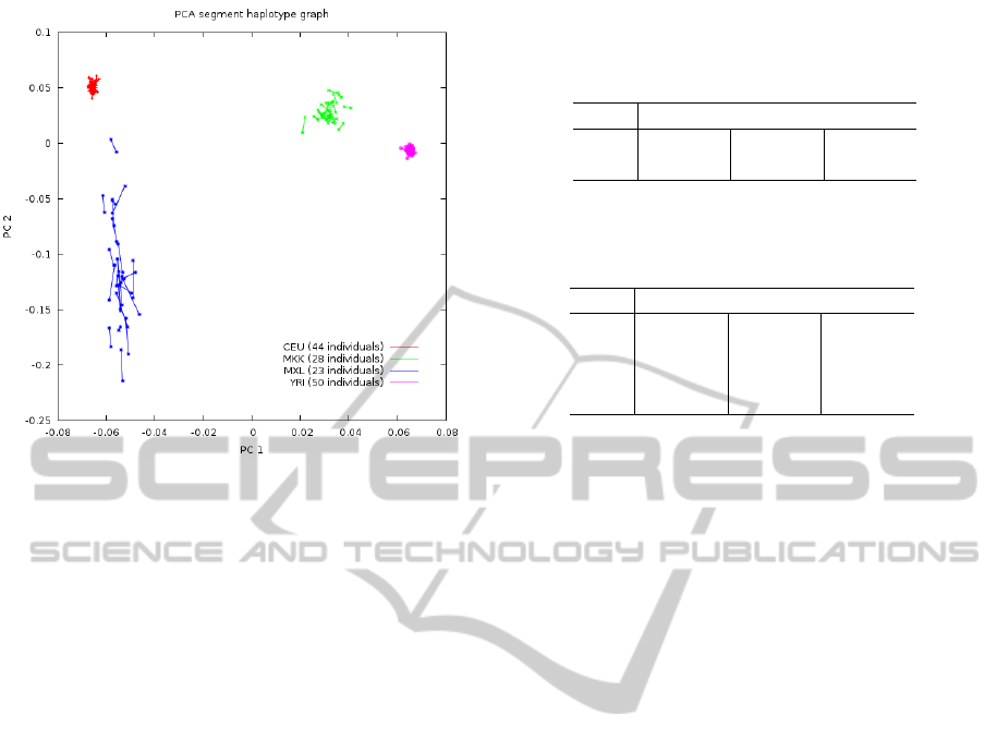
Figure 1: Phased-PC plot from HapMap samples, including
Utah residents with Northern and Western European ances-
try (CEU, red plus sign), Los Angeles residents with Mexi-
can ancestry (MXL, blue asterisks), Yoruban samples from
Ibadan (YRI, pink filled squares) and Maasai in Kinyawa
(MKK, green crosses) populations using quasi-true haplo-
types inferred from familial trios.
PCA over large data sets. Therefore, PCPhaser dupli-
cates the input genotype data in the makeped file, i.e.,
it splits each original line in the makeped file corre-
sponding to the phased genotype of an individual into
two lines, one for each haplotype, and duplicates each
allele.
Table 1 shows an example of the format of
phased genotypes for 3 SNPs and 2 individuals using
makeped (for clarity, no phenotype columns but indi-
vidual IDs are shown). The data transformation per-
formed by PCPhaser for these individuals and mark-
ers is shown in Table 2. As a result, two eigenvectors
will be produced for each individual, one for each
haplotype, which will be used by PCPhaser to draw
the segments in a phased-PC plot.
PCPhaser also allows to choose a subset of pop-
ulations to obtain the eigenvectors and the remaining
ones only to be projected on them.
As an example, Figure1 shows a phased-PC
plot produced by the method, implemented through
the software PCPhaser (http://bios.ugr.es/pcphaser).
Phased genotypes from half of the individuals pass-
ing quality control belonging to four different popula-
tions of the International Hapmap Project 3 (Hapmap
from now on) (HapMap-Consortium, 2003; HapMap-
Consortium, 2010) were randomly selected to be plot-
ted.
Table 1: Example of phased genotypes at three SNP mark-
ers for 2 individuals under the makeped format, for which
genotype-based PCA software programs (e.g. EIGEN-
SOFT) ignore the phase.
IND SNP #1 SNP #2 SNP #3
#1 C C A G C T
#2 C T G A T T
Table 2: Transformation performed by PCPhaser on phased
genotypes from Table 1 required by EIGENSOFT to carry
out phased-genotype PCA.
IND SNP #1 SNP #2 SNP #3
#1a C C A A C C
#1b C C G G T T
#2a C C G G T T
#2b T T A A T T
3 RESULTS
We have used this tool, implemented in the software
PCPhaser, to show its potential in two different re-
search lines, one related to population stratification
and admixture and the other related to methods for
haplotype resolution.
3.1 Phased PC Plots Applied to
Population Stratification and
Admixture
Phased-PC plots may be used (Figures 2 and 3) as a
tool to help uncover the level of inbreeding in differ-
ent populations. We used PCPhaser with two popu-
lations from the HapMap Project for which individ-
ual haplotypes are known –they use nuclear families
to obtain them accurately– and for which the large
difference in levels of inbreeding is already known:
MXL (30 trios, residents in Los Angeles, USA, with
Mexican ancestry) and CEU (30 trios, CEPH popula-
tion composed of Utah residents with ancestry from
Northern and Western Europe). Mexican is an ad-
mixed population with average genetic composition
of 60.70% European, 34.31% Asian (Amerindian)
and 4.99% African (Silva-Zolezzi et al., 2009) while
CEPH is a Caucasian population. From now on
we will refer to these known haplotypes as quasi-
true haplotypes since the phase cannot be completely
solved from familial trios. Thus, it remains unkown
in those positions in which all members of the family
are heterozygotic (Sebastiani et al., 2004).
To draw Figure 2 we randomly chose 44 parents
out of the 88 CEU parents from trio families avail-
able after the quality control performed by HapMap.
BIOINFORMATICS2014-InternationalConferenceonBioinformaticsModels,MethodsandAlgorithms
132
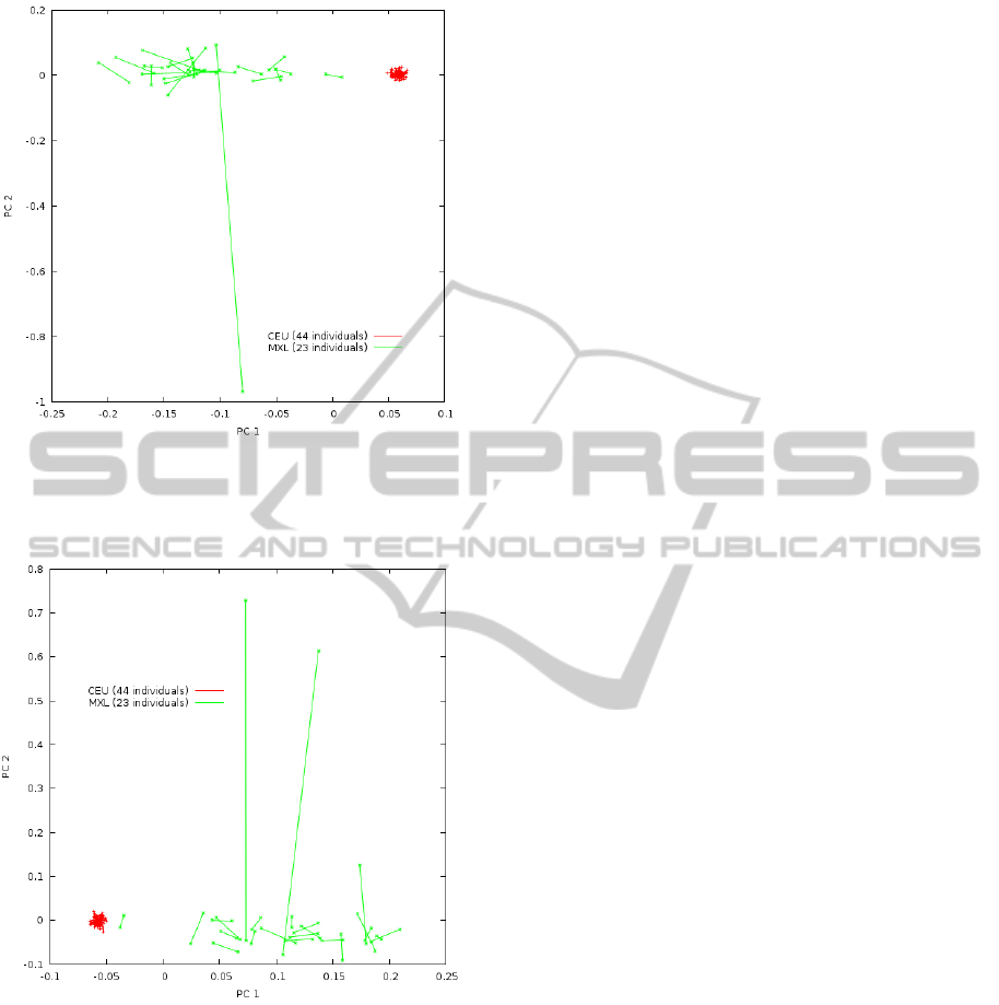
Figure 2: Phased-PC plot from HapMap MXL (green
crosses) and CEU (red plus sign) populations using quasi-
true haplotypes inferred from familial trios. The same sam-
ples used to learn the eigenvectors are plotted.
Figure 3: Phased-PC plot from HapMap MXL (green
crosses) and CEU (red plus sign) populations using quasi-
true haplotypes inferred from familial trios. Different sam-
ple subsets were used to learn the eigenvectors and to draw
the plot.
Similarly, we randomly chose 23 parents out of the
46 MXL parents from trio families available after the
quality control performed by HapMap. To draw Fig-
ure 3, once the eigenvectors were learned with the
chosen samples, the remaining samples were plotted
by projecting them on the learned eigenvectors. Both
figures show the phased-PC plots of the two first PCs
drawn by PCPhaser. Each segment represents a sin-
gle individual with the end points representing the two
haplotypes.
It must be observed the large average difference in
the segment length between MXL and CEU popula-
tions.
It must also be observed how several segments
representing MXL individuals have similar direc-
tion from/to the cluster representing CEU individu-
als to/from large values of PC1, which may reflect
the large European and Amerindian genetic compo-
sition of Mexican population. There are one (Fig-
ure 2)/two (Figure 3) individuals with very long seg-
ments orthogonal to the cluster representing the CEU
population, which may reflect they have one parent
with African ancestry (as said above, only about 5%
of Mexican genetic ancestry is from Africa) and the
other having a most common Mexican mixture of Eu-
ropean and Amerindian ancestry.
3.2 Phased PC Plots to Show Accuracy
of Algorithms for Haplotype
Reconstruction
In the second example (Figures 4, 5, 6 and 7) we have
used the method to compare the average performance
of different phasing algorithms by plotting the first 2
PCs for CEU (Figures 4 and 5) and MXL (Figures
6 and 7) populations. The main difference between
the four plots are due to the design used to perform
the analysis. Figures 4 and 6 use the same sample
subset to compute the eigenvectors and to draw the
plots, while Figures 5 and 7 use a different sample
subset to compute the eigenvectors and to draw the
plots.
In both approaches each drawn plot shows dif-
ferences between quasi-true haplotypes, two state-
of-the-art in silico methods: Beagle (Browning and
Browning, 2009) (Beagle, red plus signs) and Shape-
it (Delaneau et al., 2011) (Shapeit, green crosses)
and when haplotypes are randomly obtained, which
is equivalent to use unphased or genotype-based con-
ventional plots (Unphased, cyan filled squares).
When comparing Figures 4 and 6 it can be ob-
served how the average segment length in quasi-true
haplotypes (trios, blue asterisks) is larger in MXL
than in CEU. This is an expected result because of the
population admixture in MXL. Moreover, the advan-
tage of quasi-true haplotypes over the other methods
is clearer in MXL.
When comparing the two approaches, it can be ob-
served the large differences in the quasi-true haplo-
types (trios, blue asterisks): individual segments are
much shorter when the same samples were used to
learn the eigenvectors and to draw the plots. Con-
sidering how plot scaling changes between the plots,
SummarizingGenome-widePhasedGenotypesusingPhasedPCPlots
133
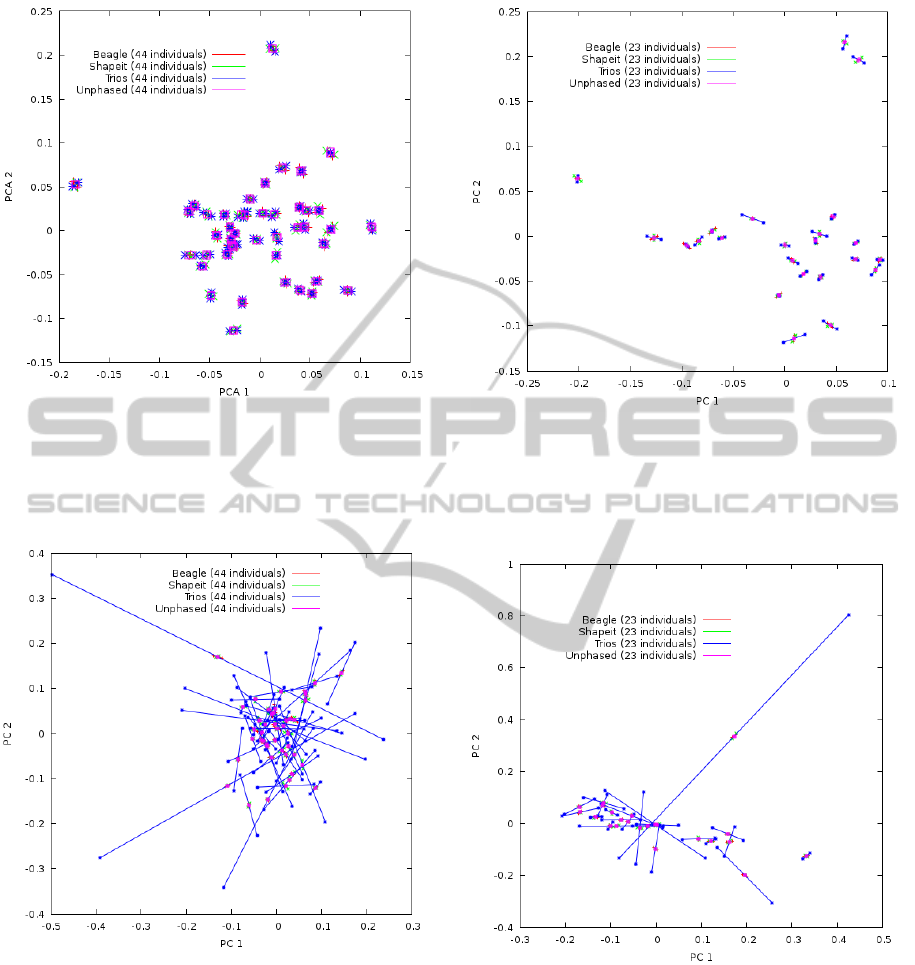
Figure 4: Phased-PC plot from CEU population using the
same panel to learn the eigenvectors and to draw the plot. 4
different methods are shown: (1) quasi-true haplotypes ob-
tained from trios (blue asterisks), Beagle (red plus signs),
Shapeit (green crosses), and random phasing (Unphased,
cyan filled squares).
Figure 5: Phased-PC plot from CEU population using an
independent panel to learn the eigenvectors. 4 different
methods are shown: (1) quasi-true haplotypes obtained
from trios (blue asterisks), Beagle (red plus signs), Shapeit
(green crosses), and random phasing (Unphased, cyan filled
squares).
this pattern is clearer in CEU. On the contrary, there
are very little differences in the other methods. This
result supports the use of the second approach since
it shows how differences increase between quasi-true
haplotypes and in-silico algorithms when an indepen-
dent sample subset was used to draw the plots.
All the plots support the idea that in-silico phas-
Figure 6: Phased-PC plot from MXL population using the
same panel to learn the eigenvectors and to draw the plot. 4
different methods are shown: (1) quasi-true haplotypes ob-
tained from trios (blue asterisks), Beagle (red plus signs),
Shapeit (green crosses), and random phasing (Unphased,
cyan filled squares).
Figure 7: Phased-PC plot from MXL population using
an independent panel to learn the eigenvectors. 4 differ-
ent methods are shown: (1) quasi-true haplotypes obtained
from trios (blue asterisks), Beagle (red plus signs), Shapeit
(green crosses), and random phasing (Unphased, cyan filled
squares).
ing methods are not accurate enough when used to
estimate long-range haplotypes, even if the algorithm
shows high accuracy rates for short-range haplotypes,
since phasing errors propagate along the chromosome
(Turner and Hurles, 2003). Moreover, when phase is
unknown or randomly solved, segments are actually
BIOINFORMATICS2014-InternationalConferenceonBioinformaticsModels,MethodsandAlgorithms
134

dots and there are no differences with the common
genotype-based PC plots.
When using the proposed method to compare ac-
curacy of different in-silico phasing algorithms, we
always need to know the true, or quasi-true, hap-
lotypes. Nowadays there are few publicly-available
data sets of true haplotypes from healthy individ-
uals. The most widely-used data sets come from
HapMap and includes quasi-true haplotypes, inferred
from familial trios, for Caucasians from Northwest
Europe (CEU), Africans from Nigeria (YRI), Kenya
(MKK, Maasai in Kinyawa) and a less-specific ori-
gin (ASW, African Ancestry in SW USA), and an ad-
mixed population (MXL, Mexican Ancestry in LA,
CA, USA). The more recent 1000 Genomes project
(Consortium’, 2010) does not include trios. There-
fore, for samples from other European or African re-
gions, or for Asian individuals it would be more diffi-
cult to find out a large enough data set of true haplo-
types to apply the proposed method.
4 CONCLUSIONS
With this work we have extended the genotype-based
PC plots to use phased genotypes and we have shown
how phased-PC plots may shed new light to this kind
of graphs helping to understand not only population
drift, stratification and admixture but also individual
genetic differences. Moreover, it may be used as a
by-view way to test accuracy of phasing methods at a
long-range haplotype level.
Based on phased-PC plots, we plan to design a
statistical test to compare accuracy between phased
genotypes returned by an in-silico phasing algorithm
and the true or quasi-true phased genotypes.
ACKNOWLEDGEMENTS
The authors were supported by projects CEI-
mic2013-2, CEI-IDi-2013-15, TIN2010-20900-C04-
1 and P08-TIC-03717 and the European Regional De-
velopment Fund (ERDF).
REFERENCES
Brisbin, A. (2010). Linkage analysis for categorical traits
and ancestry assignment in admixed individuals. PhD
thesis, Cornell University, Ithaca, New York.
Browning, B. L. and Browning, S. R. (2009). A unified ap-
proach to genotype imputation and haplotype-phase
inference for large data sets of trios and unrelated in-
dividuals. The American Journal of Human Genetics,
84(2):210–223.
Consortium’, T. . G. P. (2010). A map of human genome
variation from population-scale sequencing. Nature,
467:1061–73.
Delaneau, O., Marchini, J., and Zagury, J.-F. (2011). A
linear complexity phasing method for thousands of
genomes. Nature Methods, 9(2):179–81.
HapMap-Consortium, T. I. (2003). The international
hapmap project. Nature, 426:789–796.
HapMap-Consortium, T. I. (2010). Integrating common and
rare genetic variation in diverse human populations.
Nature, 467(7311):52–58.
Jombart, T., Pontier, D., and Dufour, A.-B. (2009). Ge-
netic markers in the playground of multivariate analy-
sis. Heredity, 102:330–41.
Lao, O., Lu, T. T., Nothnagel, M., et al. (2008). Correlation
between genetic and geographic structure in europe.
Curr. Bio., 18:1241–8.
Nicholson, G., Smith, A., Johnson, F., et al. (2002). As-
sessing population differentiation and isolation from
single-nucleotide polymorphism data. JRSS (B),
64:695–715.
Novembre, J., Toby, Bryc, K., et al. (2008). Genes mirror
geography within europe. Nature, 456(7218):98–101.
Pariset, L., Savarese, M., Cappuccio, I., and Valentini,
A. (2003). Use of microsatellites for genetic varia-
tion and imbreeding analysis in sarda sheep flocks of
central italy. Journal of Animal Breeding Genetics,
120:425–32.
Patterson, N., Price, A. L., and Reich, D. (2006). Pop-
ulation structure and eigenanalysis. PLoS Genetics,
2(12):2074–93.
Sebastiani, P., Abad-Grau, M., Alpargu, G., and Ramoni,
M. F. (2004). Robust transmission/disequilibrium
test for incomplete family genotypes. Genetics,
168(4):2329–37.
Silva-Zolezzi, I., Hidalgo-Miranda, A., Estrada-Gil, J., et al.
(2009). Analysis of genomic diversity in mexican
mestizo populations to develop genomic medicine in
mexico. PNAS, 106(21):8611–16.
Turner, D. J. and Hurles, M. E. (2003). High-throughput
haplotype determiantion over long distances by haplo-
type fusion pcr and ligation haplotyping. Nature Pro-
tocols, 4:1771–83.
Wang, C., Szpiech, Z., Degnan, J., et al. (2010). Comparing
spatial maps of human population-genetic variation
using procrustes analysis. Stat. Appl. Genet. Molec.
Biol., 9(1):13.
SummarizingGenome-widePhasedGenotypesusingPhasedPCPlots
135
