Spatial Artifact Detection for Multi-channel EMG-based Speech

Recognition

Till Heistermann, Matthias Janke, Michael Wand and Tanja Schultz

Cognitive Systems Lab, Institute for Anthropomatics, Karlsruhe Institute of Technology, Karlsruhe, Germany

Keywords:

Silent Speech Interfaces, EMG, Artifact Removal, ICA, Speech Recognition, Array Processing.

Abstract:

We introduce a spatial artifact detection method for a surface electromyography (EMG) based speech recog-

nition system. The EMG signals are recorded using grid-shaped electrode arrays afﬁxed to the speakers

face. Continuous speech recognition is performed on the basis of these signals. As the EMG data are high-

dimensional, Independent Component Analysis (ICA) can be applied to separate artifact components from the

content-bearing signal. The proposed artifact detection method classiﬁes the ICA components by their spatial

shape, which is analyzed using the spectra of the spatial patterns of the independent components. Components

identiﬁed as artifacts can then be removed. Our artifact detection method reduces the word error rates (WER)

of the recognizer signiﬁcantly. We observe a slight advantage in terms of WER over the temporal signal based

artifact detection method by (Wand et al., 2013a).

1 INTRODUCTION

Communication is the exchange of knowledge be-

tween people and thus may be considered a funda-

mental root of civilization. While there are many

ways to express thoughts and feelings, speech un-

doubtedly is the most expressive communication

method available. Furthermore, while speech evolved

as a means of face-to-face conversation among at

most a small group of persons, modern technological

enhancements, for example cell phones and speech-

based computer interfaces, have made it not only an

ubiquitous means of communication between humans

across the entire world, but also a method to control

technical devices.

This development has been a great progress, but

it also brought about problems since speech needs to

be clearly audible and cannot be shielded, resulting

in disturbance for bystanders, lack of privacy, and de-

terioration of communication in noisy environments.

Furthermore, speech-disabled persons are often ex-

cluded from using speech-based computer interfaces.

These challenges are tackled by Silent Speech Inter-

faces, which are systems enabling speech communi-

cation to take place without the necessity of emitting

an audible acoustic signal, or when an acoustic signal

is unavailable. In their survey article, (Denby et al.,

2010) provide an overview about the state of the art in

Silent Speech Interfaces, and the strengths and limita-

tions of different modalities (Electromyography, Ul-

trasound, Non-Audible Murmur, etc. ).

We report on a surface electromyography (EMG)

based Speech Recognition System, where electrical

activity of the articulatory muscles is captured by

EMG electrodes attached to the speaker’s face, and

the corresponding speech is decoded and output as

text. This method allows speech to be recognized

even when it is produced silently, i. e. mouthed with-

out any vocal effort, as demonstrated by (Jorgensen

et al., 2003). Most current approaches to EMG

based speech recognition use single electrodes for the

recording of facial electromyographic signals (Deng

et al., 2012), (Jorgensen and Dusan, 2010), (Freitas

et al., 2012). However our EMG acquisition system

uses electrode arrays, as used by (Wand et al., 2013b)

for continuous speech recognition and by (Kubo et al.,

2013) for vowel discrimination. While single elec-

trodes can be placed precisely to capture activity from

a speciﬁc muscle, they require manual setup and one

cable for every electrode. Electrode arrays capture

signals from a larger area of the speaker’s face than

single electrodes. This makes them less ﬂexible re-

garding the positioning, but allows us to locate the

exact positions of muscle activities computationally

using array processing methods. (Wand et al., 2013b)

proposed to apply Independent Component Analysis

(ICA) (Hyv

arinen and Oja, 2000) as a means to im-

prove the signal quality, and showed that the recog-

189

Heistermann T., Janke M., Wand M. and Schultz T..

Spatial Artifact Detection for Multi-channel EMG-based Speech Recognition.

DOI: 10.5220/0004793901890196

In Proceedings of the International Conference on Bio-inspired Systems and Signal Processing (BIOSIGNALS-2014), pages 189-196

ISBN: 978-989-758-011-6

 2014 SCITEPRESS (Science and Technology Publications, Lda.)

nition accuracy of the system can be improved by

extending the ICA method with an artifact removal

algorithm. ICA decomposes an N-dimensional sig-

nal into N statistically independent components. We

can interpret these components as theoretical source

signals, of which we only observe a linear superpo-

sition. The idea of artifact removal algorithms is to

take a set of ICA source components, and to heuristi-

cally separate signal from artifact components, while

keeping the signal removing the artifact components.

ICA has been used for some time to decompose EEG

signals (Jung et al., 2000), (Viola et al., 2009). Stud-

ies from medical EMG processing suggest that ICA is

also well applicable to EMG electrode arrays (Naka-

mura et al., 2004), (Ren et al., 2006). Yet to our

knowledge (Wand et al., 2013a) were the ﬁrst to use

ICA to reduce artifacts in EMG electrode array based

speech recognition. This paper improves upon that

work, which used a temporal signal based approach

to artifact detection. We study a different kind of arti-

fact detection algorithm which does not consider the

computed signal components by themselves, but di-

rectly analyzes the ICA decomposition matrix. Our

approach uses spatial information, which is comple-

mentary to the temporal information used in the tem-

poral signal based method. We therefore expect it

to detect other types of artifacts, which suggests a

possible beneﬁt from fusing these two detection ap-

proaches in future work. We show that our method

slightly outperforms, albeit not signiﬁcantly, the tem-

poral signal based method in terms of speech recog-

nition accuracy.

2 DATA CORPUS

We use the same data corpus as (Wand et al., 2013b)

and (Wand et al., 2013a), therefore we follow these

authors in the description of the recording process and

the resulting corpus. For EMG recording the EMG-

USB2 multi-channel EMG ampliﬁer was used, which

was produced and distributed by OT Bioelettronica,

Italy (www.otbioelettronica.it). The set of elec-

trode arrays was obtained from the same vendor. The

recording conﬁguration for the experiments is shown

in ﬁgure 1. Two types of arrays were used: A chin

array with a row of 8 electrodes with 5 mm inter-

electrode distance (IED), and a cheek array with 4 ×8

electrodes with 10 mm IED. In order to minimize

common-mode artifacts, a bipolar measurement con-

ﬁguration was chosen, where the potential difference

between two adjacent channels in a row was mea-

sured. This means that out of 4 × 8 cheek electrodes

and 8 chin electrodes, (4 +1) · 7 = 35 signal channels

Figure 1: Positioning of the EMG array during recording.

One 4 × 8 array is afﬁxed to the speaker’s cheek and one

1×8 array is afﬁxed underneath the chin. Image taken from

(Wand et al., 2013b) with permission.

were obtained in total. The EMG signals were sam-

pled at 2048 Hz. The audio signal was recorded with

a standard close-talking microphone in parallel to the

EMG recordings. An analog marker system was used

to synchronize the EMG and audio recordings. The

EMG signal was delayed by 50 ms compared with the

audio signal, to adjust the anticipatory properties of

EMG signal (Cavanagh and Komi, 1979) (Jou et al.,

2006).

The recording protocol follows (Schultz and

Wand, 2010): We used 7 sessions recorded by 6

speakers, where each session consisted of 50 phonet-

ically balanced English sentences: a set of 10 base

sentences, which was kept ﬁxed across sessions and

used for testing, and a set of 40 training sentences

which varied across sessions. The sentences belong

to the Broadcast News domain and were read in nor-

mal, audible speech. Note that the corpus also con-

tains larger sessions, as well as recordings of silently

mouthed speech, which were not used in this study.

All experiments were session-dependent, i. e. train-

ing and testing was performed separately for each ses-

sion. The 7 sessions have an average length of 191

seconds each, whereof 149 s are training and 42 s are

testing utterances.

3 BASELINE RECOGNITION

SYSTEM

3.1 Feature Extraction

Before any features are extracted, the data are pre-

processed by synchronizing the EMG with the audio

recordings, and by normalizing all 35 EMG channels

with respect to mean and variance. The normalization

step is necessary because of varying electrode resis-

tances at each channel.

If no Independent Component Analysis (ICA) is

applied, features are extracted from each of the chan-

nels. When ICA is applied, the ICA transformation

BIOSIGNALS2014-InternationalConferenceonBio-inspiredSystemsandSignalProcessing

190

matrix is computed session-wise on the training data,

resulting in a set of ICA components. We use the Info-

max ICA algorithm according to (Bell and Sejnowski,

1995), as implemented in the Matlab EEGLAB tool-

box (Delorme and Makeig, 2004), to compute the

ICA decomposition. For a thorough introduction to

the theory of Independent Component Analysis, we

would like to refer the reader to (Cardoso, 1998) and

(Hyv

arinen and Oja, 2000). For the subsequent ar-

tifact removal, (Wand et al., 2013a) introduced two

methods:

• The direct method means that artifact components

are removed, and features are extracted on the re-

maining ICA components.

• The back-projection method consists of taking

the ICA decomposition, setting detected artifact

channels to zero, and then applying the inverse of

the ICA transformation. This “back-projects” the

signal representation into its original domain, but

suppresses the detected noise. Features are then

extracted on the back-projected data.

We compare our results with two baseline sys-

tems: First, a baseline system without any ICA ap-

plication or artifact removal. Second, we perform the

ICA decomposition, but do not remove any compo-

nents. In all cases, features are extracted on each

channel or component separately. We use the time-

domain feature extraction proposed by (Jou et al.,

2006) and also used by (Wand et al., 2013a).

For any given frame f,

f is its frame-based time-

domain mean, P

is its frame-based power, and z

its frame-based zero-crossing rate.

For an EMG signal with normalized mean x[n],

we obtain a low-pass ﬁltered signal w[n] by using a

double nine-point moving average:

w[n] =

∑

k=−4

v[n + k] (1)

where v[n] =

∑

k=−4

x[n + k]. (2)

The complementary high-frequency signal is p[n] =

x[n] − w[n], and the rectiﬁed high-frequency signal is

r[n] = |p[n]|.

Let S(f, n) be the stacking of adjacent frames of

feature f in the size of 2n + 1 (−n to n) frames. The

feature TDn, for one EMG channel or ICA compo-

nent, is now deﬁned as follows:

TDn =S(TD0, n), (3)

where TD0 =[

w, P

, P

, z

r], (4)

i. e. a stacking of adjacent feature vectors with context

width 2 · n + 1 is performed, with varying n. Finally,

the combination of all channel-wise feature vectors

yields the TDn feature vector. Frame size and frame

shift are set to 27 ms and 10 ms, respectively.

After this step, we apply Principal Component

Analysis (PCA) on the resulting extended feature vec-

tors, reducing their dimensionality to 700. This step

is followed by Linear Discriminant Analysis (LDA)

to obtain a ﬁnal feature vector with 32 coefﬁcients.

(Wand et al., 2013b) showed that the PCA step is

necessary in order to obtain robust results: For a

small amount of training data relative to the sam-

ple dimensionality, the LDA within-scatter matrix

becomes sparse (Qiao et al., 2009), which causes

the LDA computation to become inaccurate.

LDA is a supervised method, we need to assign

classes to every feature vector of the training set. An

acoustical speech recognizer is used to align a most

likely sequence of sub-phonemes to the simultane-

ously recorded audio sequence. As the audio and

EMG data are recorded simultaneously, these sub-

phonemes can be used as classes for the EMG training

data, between which LDA maximizes discriminabil-

ity. In total, 136 different classes are used.

3.2 Training and Decoding

We perform EMG-based continuous speech recogni-

tion. For this purpose, models of words or utterances

must be constructed from smaller units. While in con-

ventional acoustic speech recognition, these units are

normally context-dependent subphones (Lee, 1989),

we follow (Schultz and Wand, 2010) and use Bun-

dled Phonetic Features (BDPFs) as foundation for

our modeling. Phonetic Features represent proper-

ties of phones, like the place or manner of articula-

tion. Phonetic feature bundling means that dependen-

cies between these features are taken into account.

Each such BDPF model is represented by a mixture

of Gaussians. The knowledge from the different pho-

netic features is merged using a multi-stream model

(Metze and Waibel, 2002) (Jou et al., 2007).

Otherwise, our recognizer follows a standard pat-

tern. We use three-state left-to-right fully continuous

Hidden Markov Models (HMM), where the emission

LDA essentially consists of a maximization problem

, where S

is the within scatter matrix and S

the between scatter matrix. The optimization is performed

by means of an eigenvalue analysis. Numerical instability

arises when the denominator of the above fraction is singu-

lar, which happens if S

has zero eigenvalues. Note that for

the PCA computation, this is not a problem since for PCA,

one maximizes a single term w

Cw (C is the sample covari-

ance matrix) instead of a fraction and all samples are used

for covariance estimation.

SpatialArtifactDetectionforMulti-channelEMG-basedSpeechRecognition

191

probabilities are modeled using multi-stream Bun-

dled Phonetic Features, as described above. Recog-

nizer training consists of generating models for non-

bundled phonetic features, running the phonetic fea-

ture bundling, and then retraining the models using

the newly generated BDPF structure. See (Schultz

and Wand, 2010) for a detailed description. For this

training, phone-based time alignments of the EMG

data are required. Since we record the acoustic speech

in parallel to the EMG data, these time-alignments

can be generated by forced-aligning the audio data

with a standard acoustic speech recognizer, according

to (Jou et al., 2006).

For decoding, we use the trained HMM together

with a trigram Broadcast News language model. The

test set perplexity is 24.24. We restrict our decoding

vocabulary to the 108 words that appear in the test set.

In this paper we follow (Wand et al., 2013a), where

the corpus which we use was ﬁrst introduced. The

small vocabulary size is due to the limited amount of

training data, it has been shown for example in (Deng

et al., 2012) that much larger vocabularies can be used

if more training data is available.

3.3 Evaluation Metric

We evaluate our recognition systems using the Word

Error Rate (WER). The Word Error Rate indicates

which percentage of spoken words is recognized

wrongly, thus lower WER values indicate better

recognition performance. It is widely used in speech

recognition. The Word Error Rate for continuous

speech recognition tasks is deﬁned as follows. The

speech recognition hypothesis and the correct refer-

ence sentence are compared by computing the optimal

alignment with respect to word-based edit distance.

Over all utterances in the test set, the number of word

substitutions (#S), insertions (#I), and deletions (#D)

is counted, and divided by the total number of words

(#T) in the references.

WER =

#S + #I + #D

. (5)

4 METHODS OF ARTIFACT

DETECTION

The goal of artifact detection algorithms is to de-

cide which ICA-components of the EMG signal rep-

resent speech-related muscle activities and which rep-

resent artifacts. We distinguish between temporal

signal based and spatial methods. In temporal sig-

nal based artifact detection, as introduced by (Wand

et al., 2013a), components are classiﬁed by the spec-

tral properties of the post-ICA signal. We introduce

spatial artifact detection as a new approach to artifact

detection for EMG arrays. Here, each independent

component is classiﬁed by the pattern of its spatial

ﬁlter, i. e. the distribution of source dimensions con-

tributing to the component. All components that are

detected as artifacts are removed before applying the

further preprocessing steps described in section 3.1.

4.1 Temporal Signal based Artifact

Detection Heuristics

In their approach to temporal signal based artifact de-

tection, (Wand et al., 2013a) designed three classiﬁca-

tion measures to recognize different kinds of artifact

signal components. All training utterances are trans-

formed separately using the ICA matrix. If at least

one of the three measures classiﬁes a component as

an artifact on more than 50%

of the training utter-

ances, this component is considered an artifact by the

temporal signal based heuristic. The authors use the

following per-utterance classiﬁcation measures:

• Autocorrelation measure: This method typically

identiﬁes regular artifacts, like power line noise.

The autocorrelation of the component signal is

computed and if the value of the ﬁrst peak exceeds

a threshold of 0.5, this component is deemed an

artifact.

• High-frequency noise detection: The surface

EMG signal has a range of 0 – 500 Hz (Zhao

and Xu, 2011). Therefore, components with dis-

tinct high-frequency parts are likely to be artifacts.

The signal is transformed into the frequency do-

main and split into a high and low frequency part

at 500 Hz. If the ratio between high-frequency

signal energy and low frequency signal energy is

larger than a threshold of 0.75, the component is

considered an artifact.

• EMG signal range: The main energy of the EMG

signal is found between 50 and 150 Hz. If the

energy of this band is less than fourfold the energy

of the remaining frequency bands, a component is

deemed an artifact.

4.2 Artifact Detection based on Spatial

Filters

We ﬁrst introduce the term spatial pattern. A spa-

tial pattern (Blankertz et al., 2008) is a matrix of the

(Wand et al., 2013a) found a consensus threshold of

50% as optimal for the direct method, and a threshold of

10% as optimal for back-projection setups.

BIOSIGNALS2014-InternationalConferenceonBio-inspiredSystemsandSignalProcessing

192

Figure 2: Typical spatial patterns for artifact components

(left) and EMG signal components (right). Red pixels indi-

cate positive channel weights and blue pixels indicate neg-

ative channel weights.

same size as the electrode array that was used for the

recording. Each spatial pattern is a compact represen-

tation of a single independent component. It is ob-

tained by remapping the column of the inverse ICA

matrix A that corresponds to the independent com-

ponent. The spatial pattern visualizes in which elec-

trodes the hidden signal component will be present by

which amount. Note that each channel can contribute

with a positive or negative weight to each component.

Figure 2 shows exemplary spatial patterns for the 28-

channel signal measured from the cheek array, where

we manually labeled the ICA components as artifacts

or EMG-like. One can see six spatial patterns, corre-

sponding to six independent components. Each spa-

tial pattern has been computed by taking one row of

the inverted ICA matrix and reshaping it into the form

of the original EMG array. The spatial patterns on

the right hand side are three typical signal compo-

nents, each exhibiting a visible region of EMG activ-

ity, with only gradually changing intensity. The left-

hand side shows three typical artifact components: Ei-

ther the spatial pattern of that component appears ran-

dom (bottom left), or the pattern is dominated by only

a few single components (top/middle left). These are

often caused by single disconnected electrodes. Note

that this observation only applies to the spatial pattern

of the cheek array: On the chin array, we observed

no direct connection between artifact components and

their spatial patterns. We assume this is because the

chin array with its eight electrodes is too small to per-

form a meaningful analysis of spatial spectra.

Using spatial patterns to visualize and classify

independent components is a common technique in

EEG applications (Blankertz et al., 2008). Viola et

al. (Viola et al., 2009) proposed a semi-automatic

technique for clustering independent components and

identiﬁcation in EEG, which is based on compar-

ing all independent components with a user-provided

template pattern, and scored them by component sim-

ilarity. We use a similar approach for classiﬁcation

of the EMG components, however we use a weaker

deﬁnition of component similarity, which also takes

position shifts of the components into account.

Given that activity of a single articulatory muscle

is usually recorded at a number of neighboring array

electrodes, we expect that good signals are likely to

originate from a whole region of the electrode array.

In contrast, many components that correspond to sig-

nal artifacts, for instance a broken channel that carries

mains hum or other noise, often originate from a sin-

gle electrode of the array.

We apply this observation to design an artifact de-

tection algorithm that prefers smooth patterns con-

taining predominantly large regions over non-smooth

patterns with frequent or abrupt changes. These two

classes can be separated well by looking at the spec-

tral domain of the spatial patterns. We therefore in-

troduce the Spatial Spectral Correlation as a measure

for image similarity and show how it can be applied

to measure the existence of smooth regions in the dis-

tributions of independent components in EMG arrays.

4.3 Spatial Spectral Correlation as a

Measure for Image Similarity

Given two image matrices I

and I

of the size M ×N,

we deﬁne the Spatial Spectral Correlation (SSC) as

the correlation between the two log-magnitude spec-

tra of the image matrices. Let

SSC(I

, I

) :=

h log|DFT

}| , log|DFT

}| i (6)

where h·, ·i denotes the scalar product of two matrices

hA, Bi =

∑

u=1

∑

v=1

u,v

· B

u,v

(7)

and DFT

{I} denotes the ﬁnite two-dimensional Dis-

crete Fourier Transform of an image matrix I ∈

M×N

DFT

{I}

u,v

N−1

∑

y=0

(

M−1

∑

x=0

x,y

· e

− j2π

) · e

− j2π

(8)

The SSC between two images is high if the images

have a similar magnitude spectrum, but low for im-

ages with diverging magnitude spectra. As this simi-

larity measure uses only the magnitude spectrum and

discards the phase information, a circular shift of the

image or any harmonic frequency does not change the

value of the SSC score, as all position information is

encoded in the phase spectrum. SSC therefore mea-

sures how well the frequency histograms of two im-

ages match.

SpatialArtifactDetectionforMulti-channelEMG-basedSpeechRecognition

193

Figure 3: The reference template for the spatial pattern of

an ideal, spatially distributed component with dominant low

frequencies. Red pixels indicate positive weights and blue

pixels indicate negative weights.

4.4 Using SSC to Select Artifact

Components

We can now use SSC to assign a score to the patterns

of the independent components. This score represents

the similarity between the magnitude spectrum of the

component’s spatial pattern and the magnitude spec-

trum template pattern. This template pattern can be

chosen to match the speciﬁc spatial patterns to look

for. For our heuristic, we chose a template pattern ad-

hoc to contain dominant low-frequency components

and only weak high-frequency components, similar

to those observed in the manually classiﬁed compo-

nents. Figure 3 shows this reference pattern.

We classify the independent components as sig-

nal or artifact components using two approaches and

compare these: The ﬁrst is an absolute threshold for

the SSC scores, the second is choosing a ﬁxed number

of high-scoring components (k-best approach). Note

that while we applied positive selection by choosing

components with high SSC to actual signal compo-

nents, one could also apply negative selection by dis-

carding components with high similarity to prototyp-

ical artifact components.

5 EXPERIMENTS AND RESULTS

We ﬁnd that the base system without ICA has an av-

erage Word Error Rate (WER) of 46.3%. If we apply

ICA without removing any components, the WER is

slightly reduced to 45.3%. We refer to this conﬁgura-

tion as ”with ICA”.

We compare the new spatial approach with the fol-

lowing reference systems: As the ﬁrst reference, we

use ”with ICA”, the best baseline setup without arti-

fact removal at a WER of 45.3%. As the second ref-

erence, we use the results of the best temporal signal

based method by (Wand et al., 2013a), using the pa-

rameters found optimal in their study. This direct tem-

poral signal based approach yields a WER of 40.8%.

From manual inspection of the data we observed

that about one third of the 28 independent compo-

nents in the cheek array correspond to artifacts. We

chose the parameters for the spatial artifact detection

heuristic accordingly: We evaluated the k-best ap-

proach choosing the 16 and 20 best-scoring compo-

nents (In ﬁgure 4, these are denoted as 16-best and 20-

best). For the absolute threshold approach, we evalu-

ated thresholds of -5 and -10 for the SSC score with

the template pattern. These thresholds classiﬁed 6.5

and 9.4 components as artifacts on average.

Note that we do not apply the spatial heuristics to

the small chin array: To ensure comparability with the

other setups, the artifact removal algorithm of (Wand

et al., 2013a) is applied to the 7 components of the

chin array. These setups were evaluated using the

recognition system described in section 3.2 on our

data corpus.

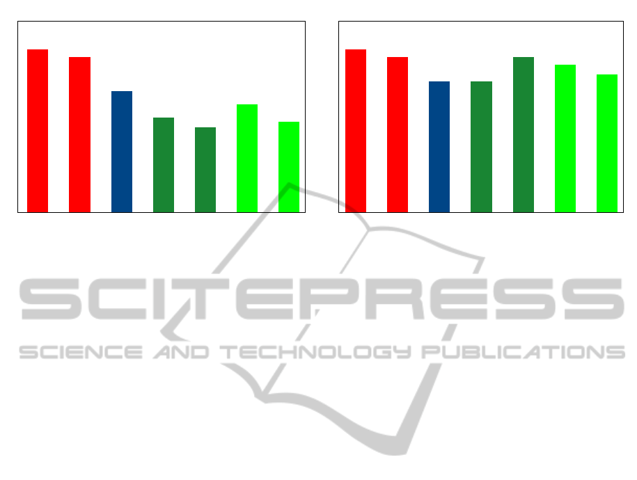
Figure 4 shows the WERs for the respective ar-

tifact reduction variants used during preprocessing.

Using direct spatial artifact detection and an absolute

SSC threshold of -5 yields a WER of 36.07%, which

is a 20.45% relative improvement compared with the

best setup without artifact removal. Compared with

the temporal signal based artifact removal method by

(Wand et al., 2013a), the WER is reduced by a relative

11.68%. Using the back-projection approach and an

SSC threshold of -10, the WER is 42.14%, which cor-

responds to a relative improvement of 7% compared

with the ”with ICA” setup. Note that the reported val-

ues of the word error rates probably overestimate the

actual improvement in WER, as the parameters for

the artifact detection method were chosen on the cor-

pus data used for evaluation. Therefore we expect a

slightly higher WER when the artifact detection is ap-

plied to yet unseen data.

All observed performance improvements were

tested for statistical signiﬁcance using paired t-tests:

For all direct spatial methods, the improvement with

respect to the ”with ICA” baseline method is signif-

icant with a conﬁdence level of > 99%. However,

when comparing the spatial with the temporal signal

based approach from (Wand et al., 2013a), the ob-

served improvement has a conﬁdence of only 85.74%,

which is not signiﬁcant. The difference between the

absolute threshold and the k-best methods for spatial

artifact detection is statistically not signiﬁcant, even

though the threshold-based methods perform slightly

better.

6 DISCUSSION

Achieving a WER of 36.1%, the artifact reduction

pushes the performance of our EMG array based

recognition system towards the range of 20 − 30%,

BIOSIGNALS2014-InternationalConferenceonBio-inspiredSystemsandSignalProcessing

194

Baseline

No ICA

Baseline

with ICA

Temporal

signal AR

Spatial AR

t=(-10)

Spatial AR

t=(-5)

Spatial AR

20 best

Spatial AR

16 best

25%

30%

35%

40%

45%

50%

46.3%

45.3%

40.8%

37.4%

36.1%

39.1%

36.8%

Average WER with direct method

Baseline

No ICA

Baseline

with ICA

Temporal

signal AR

Spatial AR

t=(-10)

Spatial AR

t=(-5)

Spatial AR

20 best

Spatial AR

16 best

25%

30%

35%

40%

45%

50%

46.3%

45.3%

42.1% 42.1%

45.3%

44.3%

43.0%

Average WER with backprojection

Figure 4: Word-Error-Rates (WER) using the direct and the back-projection method, using no artifact detection (red), temporal

signal based artifact removal (blue), spatial artifact removal with absolute thresholds (dark green), or spatial artifact removal

with k-best (light green)

which is what (Wand and Schultz, 2011) report for

the same session lengths and vocabulary sizes for sin-

gle electrode based continuous speech recognition.

Using about 7 times as much training data, (Wand

and Schultz, 2011) achieve an error rate of 10.45%.

At the same time, using about 30 times as much train-

ing data, (Deng et al., 2012) achieve an error rate of

3.1%. We thus expect that Word Error Rates for our

array based system will drop further if more training

data are used.

However, please note that it is difﬁcult to com-

pare the results of EMG based speech recognition ap-

proaches between research groups quantitatively, as

the difﬁculty of the problem at hand varies with sensor

positioning, session length, vocabulary size, the lan-

guage used and if isolated words or continuous speech

are recognized.

7 CONCLUSIONS

We have shown that the proposed spatial artifact re-

moval reduces the WER of an EMG array based

speech recognition system signiﬁcantly. Furthermore,

the spectrum of spatial patterns provides a promising

feature to classify ICA components in EMG arrays: It

discriminates spatially smooth components well from

components that consist only of a few distinct chan-

nels. The spatial method capitalizes on the continuity

of EMG signals recorded in close proximity, as op-

posed to technical artifacts which usually occur in iso-

lated channels. Our experiments show that the spatial

method performs at least as good as existing temporal

signal based artifact detection methods.

Concerning the back-projection of ICA compo-

nents vs. their direct use, we found out that the di-

rect approach is preferable. We thus conclude that the

application of an ICA transformation seems to have a

positive effect for itself, even without any removed ar-

tifacts. This conﬁrms results by (Wand et al., 2013a),

who examined the same question using their temporal

signal based artifact detection method.

REFERENCES

Bell, A. J. and Sejnowski, T. I. (1995). An Information-

Maximization Approach to Blind Separation and

Blind Deconvolution. Neural Computation, 7:1129 –

1159.

Blankertz, B., Tomioka, R., Lemm, S., Kawanabe, M., and

uller, K. (2008). Optimizing Spatial Filters for Ro-

bust EEG Single-Trial Analysis. Signal Processing

Magazine, IEEE, 25(1):41–56.

Cardoso, J.-F. (1998). Blind Signal Separation: Statistical

Principles. Proc. IEEE, 9(10):2009 – 2025.

Cavanagh, P. and Komi, P. (1979). Electromechanical Dde-

lay in Human Skeletal Muscle Under Concentric and

Eccentric Contractions. European journal of applied

physiology and occupational physiology, 42(3):159–

163.

Delorme, A. and Makeig, S. (2004). EEGLAB: An Open

Source Toolbox for Analysis of Single-Trial EEG Dy-

namics including Independent Component Analysis.

Journal of Neuroscience Methods, 134(1):9–21.

Denby, B., Schultz, T., Honda, K., Hueber, T., and Gilbert,

J. (2010). Silent Speech Interfaces. Speech Commu-

nication, 52(4):270 – 287.

Deng, Y., Colby, G., Heaton, J. T., and Meltzner, G. S.

(2012). Signal Processing Advances for the MUTE

sEMG-Based Silent Speech Recognition System. In

Military Communication Conference, MILCOM 2012,

pages 1–6. IEEE.

Freitas, J., Teixeira, A., and Dias, M. S. (2012). Towards

SpatialArtifactDetectionforMulti-channelEMG-basedSpeechRecognition

195

a Silent Speech Interface for Portuguese. In Proc.

Biosignals, pages 91 – 100.

Hyv

arinen, A. and Oja, E. (2000). Independent Component

Analysis: Algorithms and Applications. Neural Net-

works, 13:411 – 430.

Jorgensen, C. and Dusan, S. (2010). Speech Interfaces

Based Upon Surface Electromyography. Speech Com-

munication, 52:354 – 366.

Jorgensen, C., Lee, D., and Agabon, S. (2003). Sub Au-

ditory Speech Recognition Based on EMG/EPG Sig-

nals. In Proceedings of International Joint Conference

on Neural Networks (IJCNN), pages 3128 – 3133.

Jou, S.-C., Schultz, T., Walliczek, M., Kraft, F., and Waibel,

A. (2006). Towards Continuous Speech Recogni-

tion using Surface Electromyography. In Proc. Inter-

speech, pages 573 – 576.

Jou, S.-C. S., Schultz, T., and Waibel, A. (2007). Con-

tinuous Electromyographic Speech Recognition with

a Multi-Stream Decoding Architecture. In Proc.

ICASSP, pages IV–401 – IV–404.

Jung, T.-P., Makeig, S., Humphries, C., Lee, T.-W., Mcke-

own, M. J., Iragui, V., and Sejnowski, T. J. (2000). Re-

moving Electroencephalographic Artifacts by Blind

Source Separation. Psychophysiology, 37(2):163–

178.

Kubo, T., Yoshida, M., Hattori, T., and Ikeda, K. (2013).

Shift Invariant Feature Extraction for sEMG-Based

Speech Recognition With Electrode Grid. In Engi-

neering in Medicine and Biology Society (EMBC),

2013 35th Annual International Conference of the

IEEE, pages 5797–5800. IEEE.

Lee, K.-F. (1989). Automatic Speech Recognition: The De-

velopment of the SPHINX System. Kluwer Academic

Publishers.

Metze, F. and Waibel, A. (2002). A Flexible Stream Archi-

tecture for ASR Using Articulatory Features. In Proc.

ICSLP, pages 2133 – 2136.

Nakamura, H., Yoshida, M., Kotani, M., Akazawa, K., and

Moritani, T. (2004). The Application of Indepen-

dent Component Analysis to the Multi-Channel Sur-

face Electromyographic Signals for Separation of Mo-

tor Unit Action Potential Trains: Part II—Modelling

Interpretation. Journal of Electromyography and Ki-

nesiology, 14(4):433–441.

Qiao, Z., Zhou, L., and Huang, J. Z. (2009). Sparse Lin-

ear Discriminant Analysis with Applications to High

Dimensional Low Sample Size Data. International

Journal of Applied Mathematics, 39:48 – 60.

Ren, X., Hu, X., Wang, Z., and Yan, Z. (2006). MUAP

Extraction and Classiﬁcation Based on Wavelet Trans-

form and ICA for EMG Decomposition. Medical and

Biological Engineering and Computing, 44(5):371–

382.

Schultz, T. and Wand, M. (2010). Modeling Coarticulation

in Large Vocabulary EMG-based Speech Recognition.

Speech Communication, 52(4):341 – 353.

Viola, F., Thorne, J., Edmonds, B., Schneider, T., Eichele,

T., Debener, S., et al. (2009). Semi-Automatic Iden-

tiﬁcation of Independent Components Representing

EEG Artifact. Clinical Neurophysiology, 120(5):868–

877.

Wand, M., Himmelsbach, A., Heistermann, T., Janke, M.,

and Schultz, T. (2013a). Artifact Removal Algorithm

for an EMG-based Silent Speech Interface. In Proc. of

the 2013 IEEE Engineering in Medicine and Biology

35th Annual Conference.

Wand, M., Schulte, C., Janke, M., and Schultz, T. (2013b).

Array-based Electromyographic Silent Speech Inter-

face. In Proc. Biosignals.

Wand, M. and Schultz, T. (2011). Session-independent

EMG-based Speech Recognition. In Proc. Biosignals,

pages 295 – 300.

Zhao, H. and Xu, G. (2011). The Research on Surface

Electromyography Signal Effective Feature Extrac-

tion. In Proc. of the 6th International Forum on Strate-

gic Technology.

BIOSIGNALS2014-InternationalConferenceonBio-inspiredSystemsandSignalProcessing

196