Knowledge Gradient for

Multi-objective Multi-armed Bandit Algorithms

Saba Q. Yahyaa, Madalina M. Drugan and Bernard Manderick

Department of Computer Science, Vrije Universiteit Brussel, Pleinlaan 2, 1050 Brussels, Belgium

Keywords:

Multi-armed Bandit Problems, Multi-objective Optimization, Knowledge Gradient Policy.

Abstract:

We extend knowledge gradient (KG) policy for the multi-objective, multi-armed bandits problem to efﬁ-

ciently explore the Pareto optimal arms. We consider two partial order relationships to order the mean vec-

tors, i.e. Pareto and scalarized functions. Pareto KG ﬁnds the optimal arms using Pareto search, while the

scalarizations-KG transform the multi-objective arms into one-objective arm to ﬁnd the optimal arms. To

measure the performance of the proposed algorithms, we propose three regret measures. We compare the per-

formance of knowledge gradient policy with UCB1 on a multi-objective multi-armed bandits problem, where

KG outperforms UCB1.

1 INTRODUCTION

The single-objective multi-armed bandits (MABs)

problem is a sequential Markov Decision Process

(MDP) of an agent that tries to optimize its decisions

while improving its knowledge on the arms. At each

time step t, the agent pulls one arm and receives re-

ward as a feedback signal. The reward that the agent

receives is independent from the past implementa-

tions and independent from all other arms. The re-

wards are drawn from a static distribution, e.g. normal

distributions N(µ,σ

), where µ is the true mean and

is the variance. We assume that the true mean and

variance parameters are unknown to the agent. Thus,

by drawing each arm, the agent maintains estimations

of the true mean and the variance which are known as

ˆµ and

, respectively.

The goal of the agent is to minimize the loss of not

pulling the best arm i

∗

that has the maximum mean all

the time. The loss, or total expected regret, is deﬁned

for any ﬁxed time steps L as:

= Lµ

∗

−

∑

t=1

(1)

where µ

∗

= max

i=1,···,|A|

is the true mean of the

greedy (best) arm i

∗

and µ

is the true mean of the

selected arm i at time step t.

In the multi-armed bandits problem, at each time

step t, the agent either selects the arm that has

the maximum estimated mean (exploiting the greedy

arm), or selects one of the non-greedy arms in or-

der to be more conﬁdent about its estimations (ex-

ploring one of the available arms). This problem is

known as the trade-off between exploitation and ex-

ploration (Sutton and Barto, 1998). To overcome this

problem, (Yahyaa and Manderick, 2012) have com-

pared several action selection policies on the multi-

armed bandits problem (MABs) and have shown that

Knowledge Gradient (KG) policy (I.O. Ryzhov and

Frazier, 2011) outperforms other MABs techniques.

In this paper, we extend knowledge gradient

KG policy (I.O. Ryzhov and Frazier, 2011) to vec-

tor means, obtaining the Multi-Objective Knowledge

Gradient (MOKG). In the multi-objective setting,

there is a set of Pareto optimal arms that are incom-

parable, i.e. can not be classiﬁed using a designed

partial order relationship. Thus, the agent trades-

off the conﬂicting objectives (or dimensions) of the

mean vectors, the exploration (ﬁnding the Pareto front

set) and the exploitation (selecting fairly the optimal

arms).

The Pareto optimal arm set is found either by us-

ing: i) the Pareto partial order relationship (Zitzler

and et al., 2002), or ii) the scalarized functions (Eich-

felder, 2008). Pareto partial order ﬁnds the Pareto

front set by optimizing directly the multi-objective

space. The scalarized functions convert the multi-

objective space to a single-objective space, i.e. the

mean vectors are transformed in scalar values. There

are two types of scalarization functions, linear and

non-linear (or Chebyshev) functions. Linear scalar-

Q. Yahyaa S., M. Drugan M. and Manderick B..

Knowledge Gradient for Multi-objective Multi-armed Bandit Algorithms.

DOI: 10.5220/0004796600740083

In Proceedings of the 6th International Conference on Agents and Artiﬁcial Intelligence (ICAART-2014), pages 74-83

ISBN: 978-989-758-015-4

 2014 SCITEPRESS (Science and Technology Publications, Lda.)

ization function is simple and intuitive but can not

ﬁnd all the optimal arms in a non-convex Pareto front

set. In opposition, Chebyshev scalarization function

has an extra parameter to be tuned, however can ﬁnd

all the optimal arms in a non-convex Pareto front

set. Recently, (Drugan and Nowe, 2013) have used

a multi-objective version of the Upper Conﬁdence

Bound (UCB1) policy to ﬁnd the Pareto optimal arm

set (exploring) and select fairly the optimal arms (ex-

ploiting), i.e. solve the trade-off problem in the Multi-

Objective, Multi-Armed Bandits (MOMABs) prob-

lem. We compare KG policy and UCB1 on the

MOMABs problem.

The rest of the paper is organized as follows. In

Section 2 we present background information on the

algorithms and the used notation. In Section 3 we in-

troduce multi-objective, multi-armed bandits frame-

work and upper conﬁdence bound policy UCB1 in

multi-objective normal distributions bandits. In Sec-

tion 4 we introduce knowldge gradient (KG) pol-

icy and we propose Pareto knowldge gradient algo-

rithm, linear scalarized knowledge gradient across

arms algorithm, linear scalarized knowledge gradient

across dimensions algorithm, and Chebyshev scalar-

ized knowledge gradient algorithm. In Section 5 we

present scalarized multi-objective bandits. In Sec-

tion 6, we describe the experiments set up followed

by experimental results. Finally, we conclude and dis-

cuss future work.

2 BACKGROUND

In this section, we introduce the Pareto partial or-

der relationship, order relationships for scalarization

functions and regret performance measures of the

multi-objective, multi-armed bandits problem.

Let us consider the multi-objective, multi-armed

bandits (MOMABs) problem with |A|,|A| ≥ 2 arms

and with D objectives(or dimensions). Each objective

has a speciﬁc value and the objectives are conﬂicting

with each other. This means that the value of arm i can

be better than the value of arm j in one dimension and

worse than the value of arm j in other dimension.

2.1 The Pareto Partial Order

Relationship

Pareto partial order ﬁnds the Pareto optimal arm set

directly in the multi-objectivespace (Zitzler and et al.,

2002). Pareto partial order uses the following rela-

tionships between the mean vectors of two arms. We

use i and j to refer to the mean vector (estimated mean

vector or true mean vector) of arms i and j, respec-

tively:

1. Arm i dominates or is better than j, i ≻ j, if there

exists at least one dimension d for which i

≻ j

and for all other dimensions o we have i

 j

2. Arm i weakly-dominates j, i  j, if and only if

for all dimensions d, i.e. d = 1,··· ,D we have

 j

3. Arm i is incomparable with j, i k j, if and only

if there exists at least one dimension d for which

≻ j

and there exists another dimension o for

which i

≺ j

4. Arm i is not dominated by j, j ⊁ i, if and only

if there exists at least one dimension d for which

≺ i

. This means that either i ≻ j or i k j.

Using the above relationships, the Pareto optimal arm

∗

set, A

∗

⊂ A be the set of arms that are not domi-

nated by all other arms. Then:

∀

∗

∈ A

∗

, and ∀

/∈ A

∗

(∀

∈ A), we have o ⊁ a

∗

Moreover, the Pareto optimal arms A

∗

are incom-

parable with each other. Then:

∀

∗

∈ A

∗

, we have a

∗

k b

∗

2.2 The Scalarized Functions Partial

Order Relationships

In general, scalarization functions convert the multi-

objective into single-objective optimization (Eich-

felder, 2008). However, solving a multi-objective op-

timization problem means ﬁnding the Pareto front set.

Thus, we need a set of scalarized functions S to gener-

ate a variety of elements belonging to the Pareto front

set. There are two types of scalarization functions that

weigh the mean vector, linear and non-linear (Cheby-

shev) scalarization functions.

The linear scalarization assigns to each value of

the mean vector of an arm i a weight w

and the result

is the sum of these weighted mean values. The linear

scalarized across mean vector is:

(µ

) = w

+ ···+ w

(2)

where (w

,··· ,w

) is a set of predeﬁned weights

for the linear scalarized function j, j ∈ S, such that

∑

d=1

= 1 and µ

is the mean vector of arm i. The

linear scalarization is very popular because of its sim-

plicity. However, it can not ﬁnd all the arms in the

Pareto optimal set A

∗

if the corresponding mean set is

a non-convex set.

The Chebyshev scalarization beside weights,

Chebyshev scalarization has a D-dimensional refer-

ence point, i.e. z = [z

,··· ,z

]

. The Chebyshev

KnowledgeGradientforMulti-objectiveMulti-armedBanditAlgorithms

scalarized can ﬁnd all the arms in a non-convexPareto

mean front set by moving the reference point (Mietti-

nen, 1999). For maximization multi-objective multi-

armed bandits problem, the Chebyshev scalarization

is (Drugan and Nowe, 2013):

(µ

) = min

1≤d≤D

(µ

−z

), ∀

(3)

= min

1≤i≤A

−ε

, ∀

where ε is a small value, ε > 0. The reference point z

is dominated by all the optimal mean vectors. Thus,

it is the minimum of the current mean vector minus ε

value.

After transforming the multi-objective problem to

single-objective problem, the scalarized functions se-

lect the arm that has the maximum function value:

∗

= max

1≤i≤A

(µ

)

2.3 The Regret Metrics

To measure the performance of the Pareto, scalar-

ized functions partial order relationships, (Drugan and

Nowe, 2013) have proposed three regret metric crite-

ria.

1. Pareto regret metric R

Pareto

measures the distance

between a mean vector of an arm i that is pulled

at time step t and the Pareto optimal mean set.

Pareto

is calculated by ﬁnding ﬁrstly the virtual

distance dis

∗

. The virtual distance dis

∗

is deﬁned

as the minimum distance that is added to the mean

vector of the pulled arm µ

at time step t in each

dimension to create a virtual mean vector µ

∗

that

is incomparable with all the arms in Pareto set A

∗

where µ

∗

||µ

∀

i∈A

∗

as follows:

∗

= µ

+ ε

∗

where ε

∗

is a vector, ε

∗

= [dis

∗,1

,··· ,dis

∗,D

]

Then, the Pareto regret R

Pareto

is:

Pareto

= dis(µ

,µ

∗

) = dis(ε

∗

,0) (4)

where dis, dis(µ

,µ

∗

) =

∑

d=1

(µ

∗

−µ

)

is the

Euclidean distance between the mean vector of

the virtual arm µ

∗

and the mean vector of the

pulled arm µ

at time step t. Thus, the regret of the

Pareto front is 0 for optimal arms, i.e. the mean of

the optimal arm coincides itself (dis

∗

= 0 for the

arms in the Pareto front set).

2. The scalarized regret metric measures the dis-

tance between the maximum value of a scalarized

function and the scalarized value of an arm that is

pulled at time step t. Scalarized regret is the dif-

ference between the maximum value for a scalar-

ized function f

which is either Chebyshev or lin-

ear on the set of arms A and the scalarized value

for an arm k that is pulled by the scalarized f

time step t,

scalarized

(t) = max

1≤i≤A

(µ

) − f

(µ

)(t) (5)

3. The unfairness regret metric is related to the vari-

ance in drawing all the optimal arms. The unfair-

ness regret of multi-objective, multi-armed ban-

dits problem is the variance of the times the arms

in A

∗

are pulled:

unf airness

(t) =

∗

∑

∗

∈A

∗

(t) −N

∗

(t))

(6)

where R

unf airness

(t) is the unfairness regret at time

step t, |A

∗

| is the number of optimal arms, N

∗

(t)

is the number of times an optimal arm i

∗

has been

selected at time step t and N

∗

(t) is the number

of times the optimal arms, i

∗

= 1,··· , |A

∗

| have

been selected at time step t.

3 MOMABs FRAMEWORK

At each time step t, the agent selects one arm i

and receives a reward vector. The reward vector is

drawn from a normal distribution N(µ

,σ

), where

= [µ

,··· ,µ

]

is the true mean vector and σ

[σ

,··· ,µ

]

is the standard deviation vector of arm

i, and T is the transpose.

The true mean and standard deviation vectors of

arms i are unknown to the agent. Thus, by drawing

each arm i, the agent estimates the mean vector ˆµ

and

the standard deviation vector

. The agent updates

the estimated mean ˆµ

and the estimated variance

in each dimension d as follows (Powell, 2007):

i+1

= N

+ 1 (7)

ˆµ

i+1

= (1−

i+1

) ˆµ

i+1

t+1

(8)

2,d

i+1

−2

i+1

−1

2,d

i+1

t+1

− ˆµ

)

(9)

where N

is the number of times arm i has been se-

lected, ˆµ

i+1

is the updated estimated mean of arm i

for dimension d,

2,d

i+1

is the updated estimated vari-

ance of arm i for dimension d and r

t+1

is the collected

reward from arm i in the dimension d.

3.1 UCB1 in Normal MOMABs

In the single-obtimization bandits problem, upper

conﬁdence bound UCB1 policy (P. Auer and Fischer,

ICAART2014-InternationalConferenceonAgentsandArtificialIntelligence

2002) plays ﬁrstly each arm, then adds to the esti-

mated mean ˆµ of each arm i an exploration bound.

The exploration bound is an upper conﬁdence bound

which depends on the number of times arm i has been

selected. UCB1 selects the optimal arm i

∗

that maxi-

mizes the function ˆµ

2ln(t)

as follows:

∗

= max

1≤i≤A





ˆµ

2ln(t)





where N

is the number of times arm i has been pulled.

In the multi-objective multi-armed bandits prob-

lem MOMABs with Bernoulli distributions, (Drugan

and Nowe, 2013) have extended UCB1 policy to ﬁnd

the Pareto optimal arm set either by using UCB1 in

Pareto order relationship or in scalarized functions. In

this paper, we use UCB1 in the multi-objective multi-

armed bandits problem with normal distributions.

3.1.1 Pareto-UCB1 in Normal MOMABs

Pareto-UCB1 plays initially each arm i once. At each

time step t, it estimates the mean vector of each of

the multi-objective arms i, i.e. ˆµ

= [ˆµ

,··· , ˆµ

]

and

adds to each dimension an upper conﬁdence bound.

Pareto-UCB1 uses a Pareto partial order relationships,

Section 2.1 to ﬁnd the Pareto optimal arm set A

∗

UCB1

Thus, for all the non-optimal arms k /∈ A

∗

UCB1

there

exists a Pareto optimal arm j ∈A

∗

UCB1

that is not dom-

inated by the arms k:

ˆµ

2ln(t

D|A

∗

⊁ ˆµ

2ln(t

D|A

∗

Pareto-UCB1 selects uniformly, randomly one of

the arms in the set A

∗

UCB1

. The idea is to select most

of the times one of the optimal arm in the Pareto front

set, i ∈ A

∗

. An arm j /∈ A

∗

that is closer to the Pareto

front set according to metric measure is more selected

than the arm k /∈ A

∗

that is far from A

∗

3.1.2 Scalarized-UCB1 in Normal MOMABs

scalarized UCB1 adds an upper conﬁdence bound to

the pulled arm under the scalarized function j. Each

scalarized function j has associated a predeﬁned set

of weights, (w

,··· ,w

)

∑

d=1

= 1. The upper

bound depends on the number of times the scalarized

function j has been selected, N

and on the number of

times the arm i has been pulled N

under the scalar-

ized function j. Firstly, the scalarized UCB1 plays

each arm once and estimates the mean vector of each

arm, ˆµ

,i = 1, ··· , |A|. At each time step t, it pulls the

optimal arm i

∗

as follows:

∗

= max

1≤i≤A

(ˆµ

) +

2ln(N

)

where f

is either linear scalarized function, Equa-

tion 2, or Chebyshev scalarized function, Equation 3

with a predeﬁned set of weights and ˆµ

is the estimated

mean vector of arm i.

4 MULTI OBJECTIVE

KNOWLEDGE GRADIENT

Knowledge gradient (KG) policy (I.O. Ryzhov and

Frazier, 2011) is an index policy that determines for

arm i the index V

as follows:

∗x





−|

ˆµ

− max

j6=i, j∈|A|

ˆµ





where

is the Root Mean Square Er-

ror (RMSE) of the estimated mean of an arm i.

The function x(ζ) = ζΦ(ζ) + φ(ζ) where φ(ζ) =

√

2π exp(

−ζ

/2) is the standard normal density and its

cumulative distribution is Φ(ζ) =

−∞

φ(ζ

′

)dζ

′

. KG

chooses the arm i with the largest V

and it prefers

those arms about which comparativelylittle is known.

These arms are the ones whose distributions around

the estimate mean, ˆµ

have larger estimated standard

deviations,

. Thus, KG prefers an arm i over its al-

ternatives if its conﬁdence in the estimate mean ˆµ

low. This policy trades-off between exploration and

exploitation by selecting its arm i

∗

as follows:

∗

= argmax

i∈|A|



ˆµ

+ (L−t)V



(10)

where t is a time step and L is the horizon of experi-

ment which is the total number of plays that the agent

has. In (Yahyaa and Manderick, 2012), KG policy is

the competitive policy for the single-objective multi-

armed bandits problem according to the collected cu-

mulated average reward and average frequency of op-

timal selection performances. Moreover, KG policy

does not have any parameter to be tuned. Therefore,

we used KG policy in the MOMABs problem.

4.1 Pareto-KG Algorithm

Pareto order knowledge gradient (Pareto-KG) uses

the pareto partial order relationship (Zitzler and et al.,

2002) to order arms. The pseudocode of Pareto-KG

is given in Figure 1. At each time step t, Pareto-KG

calculates an exploration bound ExpB for each arm

a, (ExpB

= [ExpB

,··· ,ExpB

]

). The exploration

KnowledgeGradientforMulti-objectiveMulti-armedBanditAlgorithms

bound of arm a depends on the estimated mean of all

arms and on the estimated standard deviation of the

arm a. The exploration bound of arm a for dimension

d (ExpB

) is calculated as follows:

ExpB

= (L−t) ∗|A|D ∗v





−|

ˆµ

− max

k6=a, k∈A

ˆµ





, ∀

d∈D

where v

is the index of an arm a for dimension d, L

is the horizon of experiment which is the total num-

ber of time steps, |A| is the total number of arms, D

is the number of dimensions and

is the root mean

square error of an arm for dimension d which equals

√

. N

is the number of times arm a has been

pulled. After computing the exploration bound for

each arm, Pareto-KG sums the exploration bound of

arm a with the corresponding estimated mean. Thus,

Pareto-KG selects the optimal arms i that are not dom-

inated by all other arms k,k ∈|A|(step: 4). Pareto-KG

chooses uniformly, randomly one of the optimal arms

in A

∗

(step: 5). Where A

∗

is a set that contains

Pareto optimal arms using KG policy. After pulling

the chosen arm i, Pareto-KG algorithm, updates the

estimated mean ˆµ

vector, the estimated standard de-

viation

vector, the number of times arm i is chosen

and computes the Pareto and the unfairness regrets.

1. Input: length of trajectory

;time step

;

number of arms

|A|

;number of dimensions

;

reward distribution

r ∼ N(µ,σ

)

2. Initialize: plays each arm

Initial

steps to

estimate mean vectors

ˆµ

= [ˆµ

, ···, ˆµ

]

;

standard deviation vectors

= [

, ···,

]

3. For

t = 1

4. Find the Pareto optimal arms set

∗

such that

∀

∈ A

∗

and

∀

/∈ A

∗

ˆµ

+ ExpB

⊁ ˆµ

+ ExpB

5. Select

uniformly, randomly from

∗

6. Observe: reward vector

= [r

, ···, r

]

7. Update:

ˆµ

;

← N

+ 1

8. Compute: the unfairness regret;Pareto regret

9. End for

10. Output: Unfairness regret, Pareto regret, N.

Figure 1: Algorithm: (Pareto-KG).

4.2 Scalarized-KG Algorithm

Scalarized knowledge gradient (scalarized-KG) func-

tions convert the multi-dimensions MABs to one-

dimension MABs and make use of the estimated mean

and estimated variance.

4.2.1 Linear Scalarized-KG Across Arms

Linear scalarized-KG across arms (LS1-KG) con-

verts immediately the multi-objective estimated mean

ˆµ

and estimated standard deviation

of each arm

to one-dimension, then computes the correspond-

ing exploration bound ExpB

. At each time step

t, LS1-KG weighs both the estimated mean vector,

i.e. ([ˆµ

,··· , ˆµ

]

) and estimated variance vector,

i.e. ([

2,1

,··· ,

2,D

]

) of each arm i, converts the

multi-dimension vectors to one-dimension by sum-

ming the elements of each vector. Thus, we have

one-dimension multi armed bandits problem. KG cal-

culates for each arm, an exploration bounds which

depends on all other arms and selects the arm that

has the maximum estimated mean plus exploration

bounds. LS1-KG is as follows:

eµ

= f

(ˆµ

) = w

ˆµ

+ ···+ w

ˆµ

∀i (11)

= f

(

) = w

2,1

+ ···+ w

2,D

∀

(12)

∀

(13)





−|

eµ

− max

j6=i, j∈A

eµ





∀

(14)

where f

is a linear scalarization function that has

a predeﬁned set of weight (w

,··· ,w

), eµ

are

the modiﬁed estimated mean and variance of an arm

i, respectively which are one-dimension values and

is the modiﬁed RMSE of an arm i which is a

one-dimension value. v

is the KG index of an arm

i. x(ζ) = ζΦ(ζ) + φ(ζ) where Φ and φ are the cu-

mulative distribution and the density of the standard

normal density, respectively. Linear scalarized-KG

across arms selects the optimal arm i

∗

according to:

∗

= argmax

i=1,···,|A|

(eµ

+ ExpB

) (15)

= argmax

i=1,···,|A|

(eµ

+ (L−t) ∗|A|D ∗v

) (16)

where ExpB

is the exploration bound of arm i, |A| is

the number of arms, D is the number of dimension, L

is the horizon of an experiments, i.e. length of trajec-

tories and t is the time step.

4.2.2 Linear Scalarized-KG across Dimensions

Linear scalarized-KG across dimensions (LS2-KG)

computes the exploration bound ExpB

for each arm,

i.e. ExpB

= [ExpB

,··· ,ExpB

], adds the ExpB

ICAART2014-InternationalConferenceonAgentsandArtificialIntelligence

the corresponding estimated mean vector ˆµ

, then con-

verts the multi-objective problem to one dimension.

At each time step t, LS2-KG computes exploration

bounds for all dimensions of each arm, sums the esti-

mated mean in each dimension with its corresponding

exploration bound, weighs each dimension, then con-

verts the multi-dimension to one-dimension value by

taking the summation over each vector of each arm.

Linear scalarized-KG across dimensions is as follows:

(ˆµ

) = w

(ˆµ

+ ExpB

) + ···+ w

(ˆµ

+ ExpB

)∀

(17)

where

ExpB

= (L−t) ∗|A|D∗v

, ∀

d∈D





−|

ˆµ

− max

j6=i, j∈A

ˆµ





, ∀

d∈D

|A| is the number of arms, L is the horizon of each

experiment, v

is the index of arm i for dimension d,

ˆµ

is the estimated mean for dimension d of arm i,

is the RMSE of arm i for dimension d, ExpB

the exploration bound of arm i for dimension d and

x(ζ) = ζΦ(ζ) + φ(ζ) where Φ and φ are the cumu-

lative distribution and the density of the standard nor-

mal density, respectively. LS2-KG selects the optimal

arm i

∗

that has maximum f

(ˆµ

) as follows:

∗

= argmax

i=1,···,|A|

(ˆµ

)

4.2.3 Chebyshev Scalarized-KG

Chebyshev scalarized-KG (Cheb-KG) computes the

exploration bound of each arm in each dimension,

i.e. ExpB

= [ExpB

,··· ,ExpB

], then converts the

multi-objective problem to one-dimension problem.

Cheb-KG is as follows:

(ˆµ

) = min

1≤d≤D

(ˆµ

+ ExpB

−z

) ∀

(18)

where f

is a Chebyshev scalarization function that

has a predeﬁned set of weights (w

,··· ,w

), ExpB

is the exploration bound of arm i for dimension d

which is calculated as follows:

ExpB

= (L−t) ∗|A|D∗v

, ∀

d∈D





−|

ˆµ

− max

j6=i, j∈A

ˆµ





, ∀

d∈D

And, z = [z

,··· ,z

]

is a reference point. For each

dimension d, the corresponding reference is the min-

imum of the current estimated means of all arms mi-

nus a small positive value, ε

> 0. The reference z

for dimension d is calculated as follows:

= min

1≤i≤|A|

ˆµ

−ε

, ∀

Cheb-KG selects the optimal arm i

∗

that has maxi-

mum f

(ˆµ

) as follows:

∗

Cheb−KG

= argmax

i=1,···,|A|

(ˆµ

)

5 THE SCALARIZED

MULTI-OBJECTIEVE BANDITS

The pseudocode of the scalarized MOMABs prob-

lem (Drugan and Nowe, 2013) is given in Fig-

ure 2. Given the type of the scalarized function

f, (f is either linear-scalarized-UCB1, Chebyshev-

scalarized-UCB1, linear scalarized-KG across arms,

linear scalarized-KG across dimensions or Cheby-

shev scalarized-KG) and the scalarized function set

( f

,··· , f

) where each scalarized function f

has

different weight set, w

= (w

1,s

,··· ,w

D,s

1. Input: length of trajectory

;reward vector

r ∼ N(µ,σ

)

;type of scalarized function

;set

of scalarized function

S = ( f

, ···, f

)

2. Initialize: For

s = 1

plays each arm

Initial

steps;

observe

)

;

update:

← N

+ 1

;

← N

+ 1

;

(ˆµ

)

;

(

)

End

3. Repeat

4. Select a function

uniformly, randomly

5. Select the optimal arm

∗

that maximizes the

scalarized function

6. Observe: reward vector

∗

= [r

∗

, ···, r

∗

]

7. Update:

ˆµ

∗

;

∗

;

∗

← N

∗

+ 1

;

← N

+ 1

8. Compute: unfairness regret;scalarized regret

9. Until

10. Output: Unfairness regret;Scalarized regret.

Figure 2: Algorithm: (Scalarized multi-objective function).

The algorithm in Figure 2 plays each arm of each

scalarized function f

, Initial plays (step: 2). N

is the number of times the scalarized function f

pulled and N

is the number of times the arm i un-

der the scalarized function f

is pulled. (r

)

is the

reward of the pulled arm i which is drawn from a nor-

mal distribution N(µ, σ

) where µ is the true mean and

is the true variance of the reward. (ˆµ

)

and (

)

are the estimated mean and standard deviation vectors

of the arm i under the scalarized function s, respec-

tively. After initial playing, the algorithm chooses

randomly at uniform one of the scalarized function

(step: 4), selects the optimal arm i

∗

that maximizes

KnowledgeGradientforMulti-objectiveMulti-armedBanditAlgorithms

the type of this scalarized function (step: 5) and sim-

ulates the selected arm i

∗

. The estimated mean vector

(ˆµ

∗

)

, estimated standard deviation vector (

∗

)

, and

the number N

∗

of the selected arm and the number of

the pulled scalarized function are updated (step: 7).

This procedure is repeated until the end of playing L

steps which is the horizon of an experiment.

6 EXPERIMENTS

In this section, we experimentally compare Pareto-

UCB1, and Pareto-KG and we compare linear-

scalarized-UCB1, Chebyshev-scalarized-UCB1, lin-

ear scalarized-KG across arms, linear scalarized-KG

across dimensions, and Chebyshev scalarized-KG.

The performance measures are:

1. The percentage of time optimal arms are pulled,

i.e. the average of M experiments that optimal

arms are pulled.

2. The percentage of time each of the optimal arms

is drawn, i.e. the average of M experiments that

each one of the optimal arms is pulled.

3. The average regret at each time step which is the

average of M experiments.

4. The average unfairness regret at each time step

which is the average of M experiments.

We used the algorithm in Figure 2 for the scalar-

ized functions, and the algorithm in Figure 1 for the

Pareto-KG. To compute the Pareto regret, we need

to calculate the virtual distance. The virtual distance

dis

∗

that is added to the mean vector µ

of the pulled

arm at time step t (the pulled arm is not element in the

Pareto front (Pareto optimal arm) set A

∗

) can be calcu-

lated by ﬁrstly ranking all the Euclidean distance dis

between the mean vectors of the Pareto optimal arm

set and 0 as follows:

dis(µ

∗

,0) < dis(µ

∗

,0) < ··· < dis(µ

∗

,0)

dis

< dis

< ··· < dis

∗

where 0 is a vector, 0 = [0

,··· ,0

]

. Secondly, ﬁnd-

ing the minimum added distance dis

∗

which is calcu-

lated as follows:

dis

∗

= dis

−dis(µ

,0) (19)

where dis

is the Euclidean distance between 0 vector

and the Pareto optimal mean vector µ

∗

, and dis(µ

,0)

is the Euclidean distance between the mean vector

of the pulled arm that is not element in the Pareto

front set and vector 0. Then, add dis

∗

to the mean

vector of the pulled arm µ

to create a mean vector

that is element in the Pareto optimal mean set, i.e.

∗

= µ

+ dis

∗

and check if µ

∗

is a virtual vector that

is incomparable with the Pareto front set. If µ

∗

is in-

comparable with the mean vectors of Pareto front set,

then dis

∗

is the virtual distance, calculate the regret.

Otherwise, reduce the added distance to ﬁnd dis

∗

follows:

dis

∗

= (dis

−

dis

−dis

) −dis(µ

,0)

where D is the number of dimensions. And, check if

dis

∗

creates µ

∗

that is incomparable with the Pareto

front set. If not reduce again the dis

∗

by using dis

instead of dis

and so on.

The number of experiments M is 1000. The hori-

zon of each experiment L is 1000. The rewards

of each arm i in each dimension d, d = 1, ··· ,D

are drawn from normal distribution N(µ

,σ

i,r

) where

= [µ

,··· ,µ

]

is the true mean and σ

i,r

[σ

i,r

,··· ,σ

i,r

]

is the true standard deviation of the re-

ward. The true means and the true standard deviations

of arms are unknown parameters to the agent.

First of all, we used the same example in (Dru-

gan and Nowe, 2013) because it contains non-convex

mean vector set. The number of arms |A| equals 6,

the number of dimensions D equals 2. The stan-

dard deviation for arms in each dimension is either

equal and set to 1, 0.1, or 0.01 or different and gen-

erated from a uniform distribution over the closed

interval [0,1], i.e. taken from a normal distribu-

tion N(0.5,

/12). The true mean set vector is (µ

[0.55, 0.5]

, µ

= [0.53,0.51]

, µ

= [0.52,0.54]

= [0.5,0.57]

, µ

= [0.51,0.51]

, µ

= [0.5, 0.5]

Note that the Pareto optimal arm set (Pareto front set)

is |A

∗

| = (a

∗

) where a

∗

refers to the op-

timal arm i

∗

. The suboptimal a

is not dominated

by the two optimal arms a

∗

and a

∗

, but a

∗

and a

∗

dominates a

while a

is dominated by all the other

mean vectors. For upper conﬁdence bounce UCB1,

each arm is played initially one time, i.e. Initial = 1

as (Drugan and Nowe, 2013) (for Pareto-, linear-,

Chebyshev-UCB1), then the estimated mean of arms

are calculated and the scalarized or Pareto selection

is computed. Knowledge gradient KG needs the esti-

mated standard deviation for each arm,

, therefore,

each arm is either played initially 2 times, Initial = 2

which is the minimum number to estimate the stan-

dard deviation or each arm is considered unknown

until it is visited Initial times. If the arm is unknown,

then the estimated mean of that arm has a maximum

value, i.e. ˆµ

= max

d∈D

, ∀

j, j∈|A|

and the estimated

standard deviation, i.e.

= max

d∈D

, ∀

j, j∈|A|

increase the exploration of arms. We compare the

different setting for KG and found out that play-

ICAART2014-InternationalConferenceonAgentsandArtificialIntelligence

ing each arm initially 2 times, KG performance is

increased, therefore, we used this to compare with

UCB1. The number of Pareto optimal arms |A

∗

| is un-

known to the agent, therefore, |A

∗

| = 6. We consider

11 weight sets for the linear-, and Chebyshev-UCB1

and linear scalarized-KG across arms (LS1-KG),

linear scalarized-KG across dimensions (LS2-KG),

and Chebyshev-KG (Cheb-KG) functions, i.e. w =

{(1,0)

,(0.9, 0.1)

,··· ,(0.1,0.9)

,(0, 1)

}. For

Chebyshev-UCB1 and Chebyshev-KG, ε was gener-

ated uniformly, randomly, ε ∈ [0, 0.1].

Table 1 gives the average number ± the upper and

lower bounds of the conﬁdence interval that the opti-

mal arms are selected in column A

∗

, the average num-

ber ± the upper and lower bounds of the conﬁdence

interval that one of the optimal arm a

∗

is pulled in

columns a

∗

, a

∗

, a

∗

, and a

∗

using the scalarized func-

tions in column Functions.

Table 1 shows the number of selecting the op-

timal arms is increased by using knowledge gradi-

ent. Pareto-KG plays fairly the optimal arms. Al-

though ε set to a ﬁxed value for all the scalarized

functions set ( j = 1, ··· , 11), Chebyshev-KG per-

forms better than the linear scalarization-KG across

arms (LS1-KG) and linear scalarization-KG across

dimensions (LS2-KG ) in playing fairly the optimal

arms. While, the performance of linear scalarized-

KG across arms (LS1-KG) in playing fairly the opti-

mal arms is as same as linear scalarized-KG across

dimensions (LS2-KG). Moreover, LS1-KG prefers

the optimal arms a

∗

and a

∗

then a

∗

and a

∗

and

LS2-KG prefers the optimal arms a

∗

and a

∗

then a

∗

and a

∗

. Pareto-UCB1 performs better than linear-

and Chebyshev-scalarization-UCB1, (LS-UCB1 and

Cheb-UCB1, respectively) according to the number

of selecting optimal arms. This is the same result

in (Drugan and Nowe, 2013) when the rewards are

drawn form Bernoulli distributions. Cheb-UCB1 per-

forms better than LS-UCB1 in selecting the optimal

arms. We also see that LS-UCB1 performs better

than LS1-KG and LS2-KG in playing fairly the op-

timal arms. And, Cheb-UCB1 performs better than

Cheb-KG in playing fairly the optimal arms. Figure 3

shows the average regret performances. The x-axis is

the horizon of each experiments and the y-axis is the

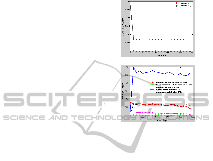
average of 1000 experiments. From Figure 3, we see

that how the regret performance is improved by us-

ing KG policy. Minimum Pareto regret is achieved by

using Pareto-KG in subﬁgure (a). Minimum scalar-

ized regret is achieved by using LS2-KG in subﬁg-

ure (b) and maximum regret is achieved by using

linear-scalarized-UCB1. From subﬁgure (b), we also

see Chebyshev-UCB1 performs better than linear-

scalarized-UCB1 and linear-scalarized-KG across di-

(a) Average Pareto regret performance

(b) Average scalarized regret performance

Figure 3: Average regret performance on bi-objective, 6-

armed bandit problems.

mensions performs better than linear scalarized-KG

across arms and Chebyshev scalarized-KG.

Secondly, we added another 14 arms to the previ-

ous example as (Drugan and Nowe, 2013). The added

arms are dominated by all other in A

∗

and have equal

mean vectors, i.e. µ

= ···µ

= [0.48,0.48]

. Fig-

ure 4 gives the average regret and the average un-

fairness regret performances of the Pareto-KG and

Pareto-UCB1. The x-axis is the horizon of each ex-

periments and the y-axis is the average of 1000 ex-

periments. Figure 4 shows the average regret perfor-

mance is improved by using Pareto-KG in subﬁgure

(a), while, the average unfairness performance in sub-

ﬁgure (b) is improved using Pareto-UCB1.

Thirdly, we added extra dimension to the previ-

ous example. The Pareto front set A

∗

contains 7

arms. Figure 5 gives the average regret performance

using σ

= 0.01. The y-axis is the average regret

performance and the x-axis is the horizon of exper-

iments. Figure 5 shows how the performance is im-

proved using KG policy in the MOMABs. Subﬁgure

a shows Pareto-KG performs Pareto UCB1. Subﬁg-

ure b shows best performance (the average regret is

decreased) for Chebyshev-KG and worst performance

for linear-UCB1. Chebyshev-UCB1 performs bet-

ter than linear-scalarized-KG across dimensions and

worse than linear-scalarized-KG across arms. And,

the Chebyshev scalarized- (KG and UCB1) is better

KnowledgeGradientforMulti-objectiveMulti-armedBanditAlgorithms

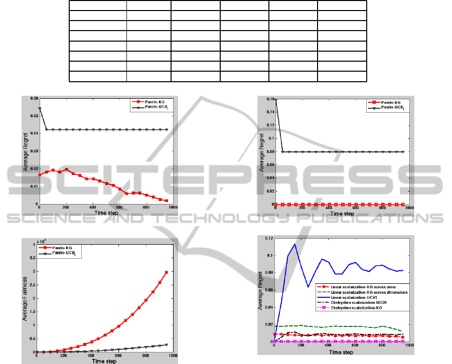
Table 1: Percentage of times optimal arms A

∗

are pulled and percentage of times each one of the optimal arm is pulled

performances on bi-objective MABs with number of arms |A| = 6 and the standard deviation of rewards are equal for each

arm i,i ∈A σ

i,r

= 0.01.

Functions A

∗

LS2-KG 999±.33 368±17.6 303±18.2 96±9.3 232±8.5

Pareto-KG 998±.02 250±.85 249±.87 250±.83 249±.82

LS1-KG 998±.04 222±9.7 122±7.4 301±14.4 353±12.2

Cheb-KG 998±.25 279±6 228±7 264±6 227±4.3

Pareto-UCB

714±.41 180±.3 163±.21 173±.23 198±.54

Cheb-UCB

677±.07 168±.08 166±.06 170±.06 173±.07

LS-UCB

669±.08 167±.06 168±.06 168±.06 166±.06

(a) Average regret performance.

(b) Average unfairness regret performance.

Figure 4: Performance comparison of Pareto-KG and

Pareto-UCB1on bi-objective MABs with 20 arms using

standard deviation of reward σ

= 0.1 for all arms. Sub-

ﬁgure (a) is the average regret performance and subﬁgure

(b) is the average unfairness regret performance.

than the linear scalarized- (KG and UCB1) according

to the regret performance.

Finally, we added extra 2 objectives in the previ-

ous triple-objective in order to compare the KG and

UCB1 performances on a more complex MOMABs

problem. Table 2 gives the average number ± the up-

per and lower bounds of the conﬁdence interval that

the optimal arms are selected in column A

∗

, the av-

erage number ± the upper and lower bounds of the

conﬁdence interval that one of the optimal arm a

∗

pulled in columns a

∗

, and a

∗

using

the scalarized functions in column Functions.

Table 2 shows the number of selecting the opti-

(a) Average Pareto regret performance

(b) Average scalarized regret performance

Figure 5: Average regret performance on triple-objective,

20-armed bandit problems.

mal arms is increased by using KG policy. Pareto-KG

outperforms Pareto-UCB1 in selecting and playing

fairly the optimal arms. Scalarized functions-KG out-

perform scalarized functions-UCB1 in selecting the

optimal arms, while scalarized functions-UCB1 out-

perform scalarized functions-KG in playing fairly the

optimal arms. LS1-KG (linear scalarized-KG across

arms) performs better than LS2-KG and Cheb-KG in

selecting the optimal arms. Cheb-KG performs bet-

ter than LS2-KG and worse than LS1-KG in select-

ing the optimal arms. LS2-KG performs better than

LS1-KG and Cheb-KG in playing fairly the optimal

arms and prefers playing a

∗

then a

∗

LS1-KG performs better than Cheb-KG and worse

than LS2-KG in playing fairly the optimal arms and

prefers a

∗

then a

∗

. Cheb-KG prefers

the optimal arms a

∗

, then a

∗

. LS-

ICAART2014-InternationalConferenceonAgentsandArtificialIntelligence

Table 2: Percentage of times optimal arms A

∗

are pulled and percentage of times each one of the optimal arm is pulled

performances on 5-objective MABs with number of arms |A| = 20 and the standard deviation of rewards are equal for each

arm i,i ∈A σ

i,r

= 0.01.

Functions A

∗

LS1-KG 1000±0 143.1±6.273 76.6±4.566 154.1±7.459 195±7.633 135.8±7.25 164.8±8.353 130.6±6.336

Cheb-KG 999.7±.023 507.3±4.111 63.6 ±4.263 111.7±4.043 29.2±3.076 73.9±4.752 193.5±4.883 20.5±2.574

LS2-KG 601.1±8.993 109.2±6.439 121.8±6.827 57.9±4.454 57.1±4.093 79.3±5.668 79.1±5.536 96.7±6.271

Pareto-KG 571.3±3.54 81.4±.723 81.7±.738 81.6±.72 81.7±.72 81.9±.688 81.6±.72 81.4±.72

Pareto-UCB

455.1±.21 64.2±.095 60.3±.066 62.7±.073 69.1±.116 65.1±.076 65.1 ±.077 68.6±.114

LS-UCB

379.7±.278 53.9±.061 53.7±.063 54.5±.064 54.7±.064 54.4±.066 54.6±.068 53.9±.066

Cheb-UCB

367.9±.219 53.4±.073 54.1±.075 52.9±.073 52.7±.075 51.9±.074 51.6±.077 51.3±.077

UCB1 and Cheb-UCB1 play fairly the optimal arms,

while LS-UCB1 performs better than Cheb-UCB1 in

selecting the optimal arms.

From the above ﬁgures and tables, we conclude

that the average regret is decreased using KG pol-

icy in the MOMABs problem. Pareto-KG outper-

forms Pareto-UCB1 and scalarized functions-KG out-

perform scalarized functions-UCB1 according to the

average regret performance. While Pareto-UCB1 out-

performs Pareto-KG according to the unfairness re-

gret, where the unfairness regret is increased using

knowledge gradient policy. However, when the num-

ber of objective is increased Pareto-KG performs bet-

ter than Pareto-UCB1 in playing fairly the optimal

arms. According to the average regret performance,

Chebyshev scalarized-KG performs better than linear

scalarized-KG across arms and dimensions when the

number of arms is increased, while LS1-KG outper-

forms all other scalarization functions when the num-

ber of objectives is increased to 5.

7 CONCLUSIONS AND FUTURE

WORK

We presented multi-objective, multi-armed bandits

problem MOMABs, the regret measures in the

MOMABs and Pareto-UCB1, linear-UCB1, and

Chebyshev-UCB1. We also presented knowledge

gradient policy KG. We proposed Pareto-KG. We

also proposed two types of linear scalarized-KG (lin-

ear scalarized-KG across arms (LS1-KG) and lin-

ear scalarized-KG across dimensions (LS2-KG) and

Chebyshev-scalarized-KG. Finally we compared KG

and UCB1 and concluded that the average regret is

improved using KG policy in the MOMABs. Fu-

ture work must provide theoretical analysis for the

KG in MOMABs and must compare the family of up-

per conﬁdence bound UCB1, and UCB1-Tuned poli-

cies (P. Auer and Fischer, 2002), and knowledge gra-

dient KG policy on the correlated MOMABs. and

must compare KG, UCB1, and UCB1-Tuned policies

in sequential ranking and selection (P.I. Frazier and

Dayanik, 2008) MOMABs.

REFERENCES

Drugan, M. and Nowe, A. (2013). Designing multi-

objective multi-armed bandits algorithms: A study. In

Proceedings of the International Joint Conference on

Neural Networks (IJCNN).

Eichfelder, G. (2008). Adaptive Scalarization Methods in

Multiobjective Optimization. Springer-Verlag Berlin

Heidelberg, 1st edition.

I.O. Ryzhov, W. P. and Frazier, P. (2011). The knowledge-

gradient policy for a general class of online learning

problems. Operation Research.

Miettinen, K. (1999). Nonlinear Multiobjective Optimiza-

tion. Springer, illustrated edition.

P. Auer, N. C.-B. and Fischer, P. (2002). Finite-time analysis

of the multiarmed bandit problem. Machine Learning,

47:235–256.

P.I. Frazier, W. P. and Dayanik, S. (2008). A knowledge-

gradient policy for sequential information collection.

SIAM J. Control and Optimization, 47(5):2410–2439.

Powell, W. B. (2007). Approximate Dynamic Program-

ming: Solving the Curses of Dimensionality. John

Wiley and Sons, New York, USA, 1st edition.

Sutton, R. and Barto, A. (1998). Reinforcement Learning:

An Introduction (Adaptive Computation and Machine

Learning). The MIT Press, Cambridge, MA, 1st edi-

tion.

Yahyaa, S. and Manderick, B. (2012). The exploration vs

exploitation trade-off in the multi-armed bandit prob-

lem: An empirical study. In Proceedings of the 20th

European Symposium on Artiﬁcial Neural Networks,

Computational Intelligence and Machine Learning

(ESANN). ESANN.

Zitzler, E. and et al. (2002). Performance assessment

of multiobjective optimizers: An analysis and re-

view. IEEE Transactions on Evolutionary Computa-

tion, 7:117–132.

KnowledgeGradientforMulti-objectiveMulti-armedBanditAlgorithms