
A User Configurable Metric for Clustering in Wireless Sensor Networks
Lina Xu, David Lillis, G. M. P. O’Hare and Rem Collier
Computer Science and Information,University College Dublin, Dublin, Ireland
Keywords:
User Configurable, Adaptation, Clustering, Voronoi.
Abstract:
Wireless Sensor Networks (WSNs) are comprised of thousands of nodes that are embedded with limited energy
resources. Clustering is a well-known technique that can be used to extend the lifetime of such a network.
However, user adaption is one criterion that is not taken into account by current clustering algorithms. Here,
the term “user” refers to application developer who will adjust their preferences based on the application
specific requirements of the service they provide to application users. In this paper, we introduce a novel
metric named Communication Distance (ComD), which can be used in clustering algorithms to measure the
relative distance between sensors in WSNs. It is tailored by user configuration and its value is computed from
real time data. These features allow clustering algorithms based on ComD to adapt to user preferences and
dynamic environments. Through experimental and theoretical studies, we seek to deduce a series of formulas
to calculate ComD from Time of Flight (ToF), Radio Signal Strength Indicator (RSSI), node density and hop
count according to some user profile.
1 INTRODUCTION
Clustering is a major approach to energy efficiency in
Wireless Sensor Networks (WSNs) (Heo and Varsh-
ney, 2005). However, most of the existing work
has focuses on energy saving, ignoring diverse re-
quirements from application developers (referred to
as “users” in this paper). They expect that the WSN
performs in a certain way that can benefit their ap-
plications the most. For example, for some applica-
tions, the user may want an immediate response in a
clustered network rather than simply reducing power
consumption. In another case, a WSN application de-
veloper may demand transmission quality more than
any other criterion. Scenarios such as these involve
a tradeoff between competing demands. Power sav-
ing is no longer an overriding factor in the system.
An advanced WSN should be sufficiently intelligent
to understand users’ preferences and thereafter adapt
as those preferences change. Currently there is little
work showing any interest in adapting user preference
in a clustering algorithm. (Liu, 2012) concludes that
Quality of Service (QoS) is neglected in current re-
search and it needs to be addressed in the future. Be-
sides energy efficiency, transmission quality and net-
work latency are two additional basic metrics used to
evaluate the QoS of a system. Voronoi diagrams (Au-
renhammer, 1991) form a fundamental data structure
for many clustering algorithms. In Voronoi cluster-
ing, Euclidean distance needs to be calculated from
the coordinates of sensors or from some other mech-
anism for representing distance.
In this paper, we motivate a novel metric—
communication distance (ComD) to substitute the
concept of Euclidean distance. A brief implementa-
tion and analysis are provided. We also discuss the
usability and alternative for ComD in real systems.
Since ComD is user configurable, clustering algo-
rithms adopting this metric are also user-configurable.
In a network, if cluster heads (CHs) are already pre-
selected randomly or through some CH election al-
gorithm, each sensor can calculate its own ComD to
every CH by using a formula that is selected based on
user configuration. Thus a sensor joining the closest
CH allows CHs to form locally optimal clusters. Us-
ing this method, ComD can evaluate and score every
single link between a sensor and a CH in the network
based on user preference. In the ideal model, every
sensor would join the CH that would render network
performance closer to the user’s preference. ComD
can overcome two particular limitations associated
with typical Voronoi-based clustering algorithms:
1. Euclidean distance cannot be used to reliably de-
termine the communication quality between sen-
sors. Even though two sensors are close to each
other geographically, their radio connection may
221
Xu L., Lillis D., M. P. O’Hare G. and Collier R..
A User Configurable Metric for Clustering in Wireless Sensor Networks.
DOI: 10.5220/0004800002210226
In Proceedings of the 3rd International Conference on Sensor Networks (SENSORNETS-2014), pages 221-226
ISBN: 978-989-758-001-7
Copyright
c
2014 SCITEPRESS (Science and Technology Publications, Lda.)

prove inadequate due to obstacles.
2. Voronoi-based approaches based on Euclidean
distance do not accommodate user preferences.
ComD reflects user preferences. Clustering algo-
rithms using ComD therefore will gain adaptive
and configurable features.
2 RELATED WORK
A wide body of research on clustering algorithms for
WSNs is available. In particular, three notable sur-
vey papers have been published (Abbasi and Younis,
2007; Boyinbode et al., 2010; Liu, 2012). Clustering
algorithms tend to focus on specific objectives, for ex-
ample, energy efficiency, load balancing or increased
scalability. However, the implications of clustering
strategies for adapting user preference have received
little attention. Individual clustering algorithms use
different metrics to decompose the network into con-
nected clusters. Examples of such metrics include
distance, hop count and cluster size (Boyinbode et al.,
2010). The metrics are pre-fixed in the clustering al-
gorithms and only fulfil certain requirements.
LEACH (Heinzelman et al., 2000) uses Radio Signal
Strength Indicator (RSSI) as a metric to cluster sen-
sors. In general, RSSI can be seen as a Link Quality
Estimator (LQE) to estimate the transmission relia-
bility. However, rather than using RSSI to guarantee
link quality, LEACH uses it from an energy reduction
perspective. Although AWARE (Urteaga et al., 2011)
concludes that it can achieve a better Packet Receive
Rate (PRR), it is not clear why this is the case. Ad-
ditionally, their clustering algorithm design does not
explicitly address the issue of reliable transmission.
(Tang and Li, 2006) provide a QoS control scheme on
a cluster-based WSN by changing data transmission
rates rather than clustering the network from a QoS
perspective. (Akkaya and Younis, 2003) introduce
a routing protocol that can find a least cost, delay-
constrained path based on a clustered WSN. (Saukh
et al., 2006) presents a generic metric for tree routing
protocols by combing two QoS metrics: 1) end-to-end
success rate and 2) resource demand. Experimental
results show that it provides considerable energy sav-
ing with equivalent end-to-end packets success rate
comparing to other metrics.
3 MOTIVATION
Clustering algorithms can organise the sensors into
clusters to achieve specific objectives. However, lit-
tle existing work incorporates a user adaptive feature.
Since different application developers have their own
preferences on the performance of a WSN, support-
ing user configurable network clustering becomes es-
sential and should be the focus of the future research.
Users view the performance of a network from three
perspectives: network latency (L), transmission relia-
bility (R) and energy consumption (C). L, R and C are
normally treated as independent measurements of a
network. However, they are intimately related to each
other and optimising for one perspective can impact
on the others. For example, if the network reliability
is improved, retransmission may be alleviated, so the
energy cost and the network latency may correspond-
ingly be reduced.
Our goal is to develop a new metric ComD that ac-
counts for all three perspectives both individually and
jointly. It measures the logical distance between sen-
sors and can be used in Voronoi clustering to substi-
tute the concept of physical distance (Euclidean dis-
tance). Each user configuration constructs a unique
non-Euclidean space. The ComD of the same link in
different spaces can have different values. The value
of ComD determines how close the performance of
a given connection can be to the user’s requirements.
If a link between two sensors is close to the user re-
quirement, the logical distance is short and vice versa.
While the physical sensor network is fixed, the log-
ical structure transforms in different spaces accord-
ing to user preference. This metric allows a WSN
to dynamically re-cluster itself as user requirements
change. This will be achieved by designing ComD to
be a user-aware measure of the quality of a link be-
tween two sensor nodes. In order to achieve this, we
must first decompose L, R and C and understand their
underlying interrelationships in more detail.
4 ANALYSIS AND EXPERIMENT
ON ComD
4.1 Overview of ComD
Since the value of ComD is entirely determined by
user configuration on the QoS criteria (L stands for la-
tency, R stands for reliability and C stands for power
consumption), different calculation formulae should
be considered for different cases, as shown in Table 1.
L can be set to be low to indicate a design for low la-
tency. If there are no constraints on L, it will be set
to 0. It is the same situation with R and C. 7 dif-
ferent configurations are available. The configuration
(0,0,0) is not considered since it means there is no
constraint on the network performance. ComD for
SENSORNETS2014-InternationalConferenceonSensorNetworks
222

Table 1: User configurations (ComD column reflects the
formulae in the following sections).
Case L R C ComD
C
1
0 0 Low (3)
C
2
0 High 0 1/(2)
C
3
0 High Low TBC
C
4
Low 0 0 (1)
C
5
Low 0 Low TBC
C
6
Low High 0 TBC
C
7
Low High Low TBC
configuration C
1
, C
2
and C
4
are guaranteed fixed for-
mulae that will be presented in the following sections
based on experiments. Other cases requiring com-
binations of criteria are marked “TBC” and will be
addressed in future work. Equation (1) (2) and (3)
present the calculations for L, R and C. The calcu-
lation formula of ComD for configuration C
2
is the
reciprocal of Equation ( 2). The reason is that the
higher transmission quality between two sensors, the
shorter ComD should be. For other cases, since there
is a tradeoff between different criteria, to simplify our
problem, we set equal priority to each of them.
We believe that L, R and C are determined by ser-
val common factors: hop count, radio signal strength
(RSSI), time of flight (ToF) and node density. RSSI
can indicate link quality between sensors. Since net-
work latency is measured at the user end, ToF in this
paper specifically refers to application level commu-
nication time rather than hardware signal level. ToF
reflects the time delay on a link. A communication
path may be formed by several links, therefore hop
count is also considered. To reveal the relationship
between the three metrics, we need to discover how
these factors influence each of the QoS metrics.
4.2 Network Assumptions
Several assumptions are made:
1. The Base Station (BS) is placed far from the sens-
ing field. It is assumed to exhibit 100% reliability.
2. Each sensor has a fixed location and only belongs
to a single cluster at any point. Sensors can con-
nect to their CHs through single or multi-hop.
3. All the sensors, including the CHs, adopt a first-
come-first-served (FCFS) processing pattern.
4. When the WSN starts, every sensor broadcasts its
own information to its neighbours and records the
RSSI, ToF from its neighbours.
Since limited work is focusing on application level
ToF, it needs careful investigation. In contrast, a lot of
research has examined the relationship between RSSI,
transmission power and link quality, so our analysis
for this area is partially founded on the existing work
(Baccour et al., 2012).
4.3 Network Latency
Network latency depends on the communication de-
lay between two sensors, which can be influenced
by several factors (e.g. distance or sensor process-
ing ability). Application-level ToF not only reveals
the communication time spent over the air, but also
the processing time on a sensor. Therefore it is highly
related to network latency.
To examine network latency, experiments were con-
ducted using SunSPOT nodes (Smith, 2007) embed-
ded with the CC2420 radio chip. All the nodes are
time synchronised to simplify the test. Otherwise,
round-trip time would be required. To investigate the
relationship between application level ToF and dis-
tance in an office area, experiments were performed
by varying the transmitter’s location between 1 me-
tre and 35 metres. The transmitter created a connec-
tion with the receiver at 1 m. it was then moved
in 1 m interval, with the average ToF value for 10
packets recorded each time. The results from two re-
peated experiments are shown in Figure 1. This il-
lustrates that there are no major differences for ToF if
distance < 21m. When distance > 21m, ToF is unpre-
dictable and unstable. This is because the link quality
is weak and retransmission frequently occurs. Due to
the establishment of the connection, the ToF of the
first packet is slightly longer. As we can see, when
retransmission does not occur, distance will not af-
fect application level ToF. The major reason is that the
time spent over air is too slight to be reflected on ap-
plication level ToF. We conclude therefore that physi-
cal distance is not an important factor in determining
network latency (L).
Figure 1: Single hop application level ToF for different dis-
tance.
In the above experiments, the measured ToF is based
on a single hop. However, a sensor may need more
than one hop to communicate with a certain CH. This
AUserConfigurableMetricforClusteringinWirelessSensorNetworks
223
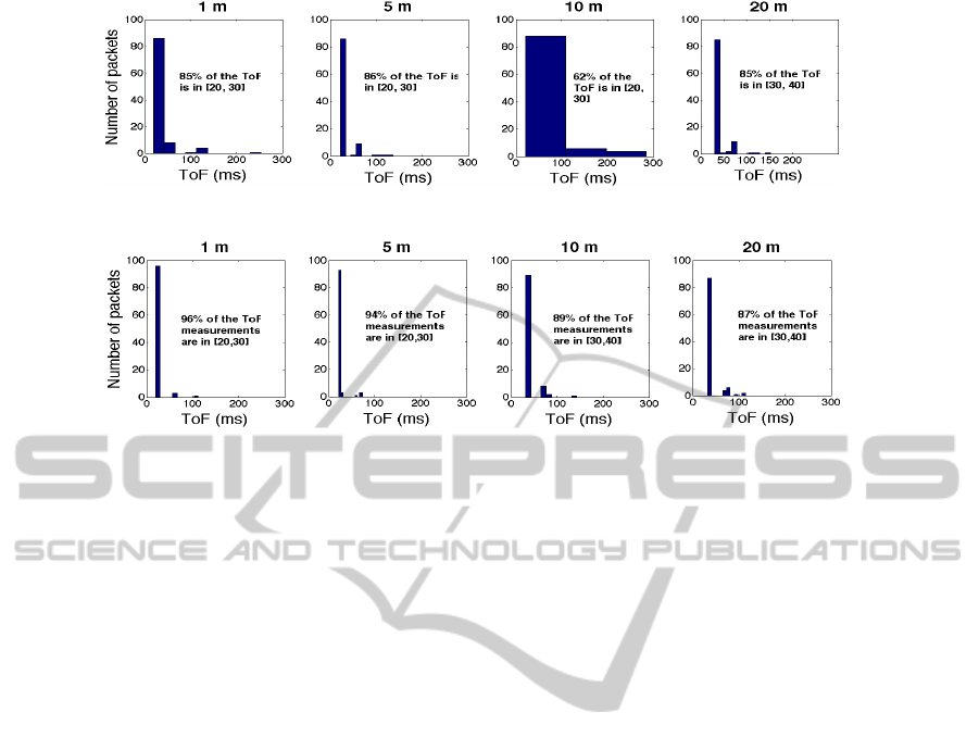
Figure 2: Experiment 1: S
1m
, S
5m
and S
10m
need single hop to the receiver, S
20m
needs 2 hops with the transit from S
5m
.
Figure 3: Experiment 2: S
10m
was changed from single hop to 2 hops with transit from S
1m
. Other conditions keep the same
as in experiment 1.
motivates a further experiment in order to discover
the relationship between the number of hops and ToF.
The relationship helps to estimate the overall ToF of
an entire path based on the ToF of each single link
and hop counts. Four transmitters (S
1m
, S
5m
, S
10m
and S
20m
) were placed at fixed locations (1, 5, 10 and
20 meters) and each of them sent 100 packets to the
BS, within 1 or 2 hops (S
1m
, S
5m
and S
10m
were con-
figured for 1 hop, while S
20m
required 2 hops). In
experiment 1, as shown in Figure 2, S
1m
and S
5m
’s
ToF is mostly in the range [20,30] ms, while S
10m
’s
ToF has a somewhat larger range [20, 100] ms with a
standard deviation (STD) of 126.8ms because its con-
nection quality is not comparable with those at S
1m
or
S
5m
, which necessitates retransmission. However, for
single hop communication, the communication time
predominantly stays within [20,30] ms. S
20m
’s 2-hop
ToF is mostly in [30,40] ms range, longer than a sin-
gle hop but less than twice of it.
In experiment 2, S
10m
was changed from a single
hop to 2-hop with all other variables being held con-
stant. Following this, its ToF is increased to the range
[30,40] ms with the STD of 16.9ms. The reason for
lower STD is that the 2-hop connection is more reli-
able than the single hop and retransmission is allevi-
ated. The ToF of the other sensors stays in a similar
range as in experiment 1. If the link quality is poor,
retransmission will occur. In such a case, from the
user perspective, the required data is delayed. This
represents a further reason why we choose applica-
tion level ToF, since it is related to link quality and
can reflect the time cost on retransmission.
The multi-hop experiment confirms the conclusion
drawn from the single link experiment namely that
distance has limited effect on application level ToF.
However, due to that the noise level changed in the
same environment, retransmission rate at 10 m is
higher than the results that are observed from the sin-
gle link experiment. The network delay is influenced
by multi-hop ToF that is determined by single hop
ToF and hop counts. In a real network, sensors can
only transmit data when the channel is clear, which
means that no other transmitter is using that channel.
As a result, the local density of the CH will also affect
the network latency (Kim et al., 2012). The network
delay between two sensors can be presented as a func-
tion of ToF, hop count and node density:
L = l (ToF,Hops,Density). (1)
4.4 Transmission Reliability
A packet can reach the receiver successfully only
when the over-air connection (the link) between two
sensors is reliable and the receiver’s buffer is not full
(Yousefi et al., 2010). RSSI has been proven to be a
good link quality estimator over a reasonable amount
of measurements (Baccour et al., 2012). It exhibits
a high correlation with PRR and it is more efficient
than PRR. In our office environment, the relation-
ship between RSSI and PRR is investigated through
experiments and the result is illustrated in Figure 4.
In ComD, we can use RSSI as a link quality metric.
Adopting the same idea as (Lin et al., 2006), if the
RSSI is over a specified threshold, we can assume that
the link is transmission reliable. This threshold is re-
lated to the environment, hardware and the required
quality. From the experiment in Section 4.3 we can
see that retransmission can be reflected in the applica-
SENSORNETS2014-InternationalConferenceonSensorNetworks
224
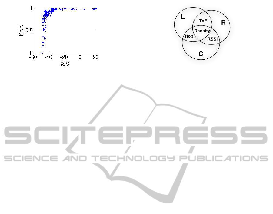
Figure 4: The relationship between RSSI and PRR.
tion level ToF. Meanwhile retransmission reveals poor
link quality. Therefore we believe that ToF can also
act as a proxy for link quality. Using the combination
of ToF and RSSI can address the link quality better. A
packet can be received only when the receiver’s buffer
is not full. The probability of overflow is determined
by data load, which depends on node density (Klein-
rock, 1975). However, the model is not practical in
real system since the receiving rate from all sources is
hard to measure before the network structure is final
formed. The idea of predicting receiving rate from lo-
cal density is used. Hence in order to determine the
transmission reliability between two sensors, we use
a function that combines ToF, RSSI and node density:
R = r (RSSI, ToF, Density). (2)
4.5 Energy Cost
A clustering algorithm normally can save power for a
network in two distinct ways: One way is through the
clustered structure. A CH can assemble the data from
each sensor in the cluster and then send the assem-
bled data to the BS. This saves energy through reduc-
ing the power consumption of transmission of each
individual sensor. However, it increases the overhead
of the CHs. In some extreme cases, some clusters
are much larger than others. The CHs of these larger
clusters will die earlier. As a result, the sensors in a
WSN should be distributed to each CH evenly, to bal-
ance the power usage. The node density surrounding
a CH will dictate the number of sensors that join the
cluster. Thus node density is a consideration when
determining energy cost. Additionally, (Wang et al.,
2006) indicates that multi-hop consumes more energy
than single hop under realistic circumstances. There-
fore sensors joining a CH through fewer hops can also
save more energy. The other way is through transmis-
sion power control. If the RSSI between two sensors
is higher than a threshold, the transmitter can lower
its transmission power to reduce the transmission cost
while maintaining the link quality. The threshold
erases the problem that when decreasing the transmis-
sion power, link quality becomes poor. This technique
Figure 5: Users view network latency (L), reliability (R)
and power consumption (C) as independent objectives, but
they are highly coupled.
is called transmission power control. More power can
be saved if the RSSI is higher (Lin et al., 2006). For
the above reasons, the energy cost for the communi-
cation between two sensors can be expressed as:
C = c (Density, Hops, RSSI). (3)
4.6 Multi-choice User Case
The relationship between network latency (L), reli-
ability (R) and power consumption (C) is shown in
Figure 5. Three of them are highly related to each
other and they can be determined by four factors in-
cluding local node density, ToF, hop count and RSSI.
However, how significantly the four factors can affect
each of the three criteria is unequal. For configura-
tion C
1
, C
2
and C
4
in Table 1, the user only have one
single requirement. Therefore we can simply assign
ComD to C, 1/R (The higher the transmission relia-
bility is between two sensors, the shorter ComD ought
to be.) or L. For other multi-selection user configura-
tions, it is necessary to combine two or three metrics
to calculate ComD and this needs careful investiga-
tion. By default, we can assume that the user puts
equal weight on each criterion. One naive proposal
is to multiply the corresponding metrics. For exam-
ple, as C
3
combines C
1
(C) and C
2
(1/R), it can be
represented as ComD = C/R. The problem is that the
domains of function l, r, and c may demand the deter-
mination and application of some coefficients for nor-
malisation. Furthermore, if RSSI affects C in a linear
manner while affecting R in a experimental manner,
when RSSI changes, R changes quicker than C. Con-
sequently, R may dominate the combination value.
Then the combination configuration will have an un-
even priority on C and R. For the above reasons, the
multi-choice user cases still need further study.
5 DISCUSSION
In this paper, we choose four factors including ToF,
hop count, RSSI and node density to characterize net-
AUserConfigurableMetricforClusteringinWirelessSensorNetworks
225

work latency (L), reliability (R) and power consump-
tion (C). Although other factors can also be used,
there are several reasons supporting our choice:
1. The selected factors are easy to capture. Through
the broadcasting in the initial phase, ToF, RSSI
and local density can be known. The hop count
from a sensor to a CH is available from the packets
received from the CH.
2. The protocol only relies on communication infor-
mation. It is not necessary to know the physical
locations of the sensors, which cannot be easily
measured by the sensors themselves.
3. The measured values are obtained from real time
data, which makes ComD adaptive to a change-
able environment.
Currently the user configuration of L, R and C is a bi-
nary choice. As we have mentioned in Section 4.1, for
the combination cases, we set equal priority to each
criterion. In the future, it will be implemented in a
manner that an application developer can put differ-
ent weight on the three metrics.
To support multi-hop communication in a cluster, not
only the CHs need to broadcast their information, but
also some other sensors. We call this process the
second-level broadcast. Deciding the number of sen-
sors that should perform second-level broadcasting is
a non-trivial problem. If there are not enough sen-
sors to broadcast, some sensors may be not able to
discover a multi-hop route.
6 CONCLUSIONS AND FUTURE
WORK
This paper provides a novel user-configurable met-
ric that facilitates user adaption in clustering algo-
rithms for WSNs. This metric is influenced by and
accommodates three performance objectives that nor-
mally exercise users in a WSN, namely: network la-
tency, transmission quality and energy consumption.
The underlying relationship between these three op-
erational parameters is revealed. In the future, more
work will be undertaken in the analysis of the inter-
relationship between these aspects so as to construct
a formula that balances them within a user configura-
tion. The performance of ComD will be evaluated in
both simulation and real time experiments.
REFERENCES
Abbasi, A. A. and Younis, M. (2007). A survey on clus-
tering algorithms for wireless sensor networks. Com-
puter Communications, 30(1415):2826 – 2841.
Akkaya, K. and Younis, M. (2003). An energy-aware qos
routing protocol for wireless sensor networks. In Dis-
tributed Computing Systems Workshops.
Aurenhammer, F. (1991). Voronoi diagrams: a survey of a
fundamental geometric data structure. ACM Comput.
Surv., 23.
Baccour, N., Koub
ˆ
aa, A., Mottola, L., Z
´
u
˜
niga, M. A.,
Youssef, H., Boano, C. A., and Alves, M. (2012).
Radio link quality estimation in wireless sensor net-
works: A survey. Trans. Sen. Netw.
Boyinbode, O., Le, H., Mbogho, A., Takizawa, M., and Po-
liah, R. (2010). A survey on clustering algorithms for
wireless sensor networks. In Network-Based Informa-
tion Systems, pages 358–364.
Heinzelman, W., Chandrakasan, A., and Balakrishnan, H.
(2000). Energy-efficient communication protocol for
wireless microsensor networks. In HICSS.
Heo, N. and Varshney, P. (2005). Energy-efficient deploy-
ment of intelligent mobile sensor networks. Systems,
Man and Cybernetics, 35(1):78–92.
Kim, D., Abay, B., Uma, R. N., Wu, W., Wang, W., and
Tokuta, A. (2012). Minimizing data collection latency
in wireless sensor network with multiple mobile ele-
ments. In INFOCOM, 2012 Proceedings IEEE.
Kleinrock, L. (1975). Theory, Volume 1, Queueing Systems.
Wiley-Interscience.
Lin, S., Zhang, J., Zhou, G., Gu, L., Stankovic, J. A., and
He, T. (2006). Atpc: adaptive transmission power con-
trol for wireless sensor networks. In Embedded net-
worked sensor systems. ACM.
Liu, X. (2012). A survey on clustering routing protocols in
wireless sensor networks. Sensors, 12(8).
Saukh, O., Marrn, P., Lachenmann, A., Gauger, M., Minder,
D., and Rothermel, K. (2006). Generic routing met-
ric and policies for wsns. In Rmer, K., Karl, H., and
Mattern, F., editors, Wireless Sensor Networks, vol-
ume 3868 of Lecture Notes in Computer Science.
Smith, R. B. (2007). Spotworld and the sun spot. In Pro-
ceedings of the 6th international conference on Infor-
mation processing in sensor networks, IPSN. ACM.
Tang, S. and Li, W. (2006). Qos supporting and optimal
energy allocation for a cluster based wireless sensor
network. Computer Communications, 29(1314).
Urteaga, I., Yu, N., Hubbell, N., and Han, Q. (2011). Aware:
Activity aware network clustering for wireless sensor
networks. In Local Computer Networks (LCN).
Wang, Q., Hempstead, M., and Yang, W. (2006). A realis-
tic power consumption model for wireless sensor net-
work devices. In Sensor and Ad Hoc Communications
and Networks, volume 1.
Yousefi, H., Mizanian, K., and Jahangir, A. (2010). Model-
ing and evaluating the reliability of cluster-based wire-
less sensor networks. In Advanced Information Net-
working and Applications.
SENSORNETS2014-InternationalConferenceonSensorNetworks
226
