Advanced EEG Processing for the Detection of Drowsiness in Drivers

Griet Goovaerts

1,2

, Ad Denissen

, Milica Milosevic

1,2

, Geert van Boxtel

and Sabine Van Huffel

1,2

KU Leuven, Department of Electrical Engineering (ESAT), STADIUS Center for Dynamical Systems,

Signal Processing and Data Analytics, Leuven, Belgium

iMinds Future Health Department, Belgium

Brain, Body and Behavior Group, Philips Research, Eindhoven, The Netherlands

Department for Psychology, Tilburg University, Tilburg, The Netherlands

Keywords:

EEG, Drowsiness Detection, Blind Source Separation.

Abstract:

Drowsiness is a serious problem for drivers which causes many accidents every day. It is estimated that drowsi-

ness is the cause of four deaths and 100 injuries per day in the United States. In this paper two methods have

been developed to detect drowsiness based on features of ocular artifacts in EEG signals. The ocular artifacts

are derived from the EEG signals by using Canonical Correlation Analysis (BSS-CCA). Wavelet transforms

are used to automatically select components containing eye blinks. Sixteen features are then calculated from

the eye blink and used for drowsiness detection. The ﬁrst method is based on linear regression, the second on

fuzzy detection. For the ﬁrst method, the drowsiness level is correctly detected in 72% of the epochs. The sec-

ond method uses fuzzy detection and detects the drowsiness correctly in 65% of the epochs. The best results

are obtained when using one single eye blink feature.

1 INTRODUCTION

Drowsiness is the strong desire to sleep felt before

actually falling asleep (Geetha and Geethalakshmi,

2011). When someone is drowsy, he is less alert and

will perform less efﬁciently tasks that require a lot

of concentration (Borghini et al., 2012). It is a nat-

ural process which normally causes no extraordinary

problems but it can be dangerous while performing

a task that requires mental attention such as driving.

Drowsy drivers are estimated to be the cause of 7%

of all trafﬁc accidents. Additionally, 16% of all acci-

dents with at least one casualty involve a tired driver

(A.A.A. Foundation, 2010), causing more than four

deaths and 100 injuries per day in the United States

(Borghini et al., 2012). Interviews with drivers indi-

cate that, while they are not aware of the moment they

fall asleep, they are aware of the fact that they are be-

coming drowsy (Reyner and Horne, 1998). Detect-

ing the level of drowsiness and giving an alarm sig-

nal when this level becomes too high would thus be a

way to decrease the number of accidents and danger-

ous situations caused by drowsy driving.

Drowsiness has an effect on many physiological

parameters, such as EEG rhythms, heart rate vari-

ability and EOG signals (Borghini et al., 2012). For

drowsiness detection in drivers, the best base for de-

tection is the use of EOG signals. (Borghini et al.,

2012) indicate that characteristics of EOG signals sig-

niﬁcantly change while performing a task that re-

quires visual attention such as driving. Often, features

such as velocity, duration and amplitude are derived

from the EOG signal and variations in those features

are used to detect drowsiness (Yue, 2011) (Svensson,

2004) (Picot et al., 2011). Different detection ap-

proaches have been used, using for example Support

Vector Machines (Hu and Zheng, 2009), multiple re-

gression (Verwey and Zaidel, 2000) and artiﬁcial neu-

ral networks (Vuckovic et al., 2002). In this paper

a simpler approach using linear regression and fuzzy

detection is explored. The validation of drowsiness

detection is done by comparing the detected drowsi-

ness level with a subjective rating given by the subject

himself. The rating can be given on the Karolinska

sleepiness scale (KSS) (Kaida et al., 2006) which has

values from one to nine. Often, a scale with less gra-

dations is used to make detection easier.

In this paper, drowsiness is detected using the ocu-

lar artifacts present in the EEG signal. The brain sig-

nal is ﬁrst separated from the artifact signal using a

blind source separation method. Out of all BSS meth-

ods, Canonical Correlation Analysis is chosen (BSS-

205

Goovaerts G., Denissen A., Milosevic M., van Boxtel G. and Van Huffel S..

Advanced EEG Processing for the Detection of Drowsiness in Drivers.

DOI: 10.5220/0004800102050212

In Proceedings of the International Conference on Bio-inspired Systems and Signal Processing (BIOSIGNALS-2014), pages 205-212

ISBN: 978-989-758-011-6

 2014 SCITEPRESS (Science and Technology Publications, Lda.)

CCA), since (Vergult et al., 2007) and (Borga and

Knutsson, 2001) show that CCA performs better in

separating brain and muscle signals and equally well

for brain and ocular signals than alternatives such as

ICA. Furthermore, it performs an order of a magni-

tude faster than ICA (Borga and Knutsson, 2001).

2 DATA COLLECTION

The data used in this project are obtained from an

experiment that was conducted by Philips Research

in collaboration with the Dutch Organization for Ap-

plied Scientiﬁc Research (TNO) in February 2011.

20 male experienced drivers and 7 back-up sub-

jects between 25 and 45 years old were selected and

had to be present in the testing center for one full day.

During this day they ﬁnished three different drives in

a driving simulator and ﬁlled in a number of ques-

tionnaires about their sleep quality. In the morning,

the participant drove for one hour in the simulator.

During this time, the baseline measurement was per-

formed: a measurement of the participant’s biosig-

nals when he is alert. In the afternoon session, two

more drives of 3.5 hours had to be ﬁnished where the

participant was driving in monotonous trafﬁc condi-

tions. Every 5 minutes a questionnaire appeared on

the screen where the subject had to indicate his state

of alertness at that moment.

Different types of signals are recorded throughout

the experiment. The ﬁrst type are biosignals. They in-

clude EEG, EOG, heart rate and respiration measure-

ments. The sampling rate of all biosignals is 1024 Hz.

The EEG signals were measured with 32 electrodes

using the International 10-20 system (Homan et al.,

1987). In addition, the user perception questionnaires

assess how tired the subject feels. The Karolinska

sleepiness scale is used, a 9-graded scale with 1 being

extremely alert and 9 extremely sleepy (Kaida et al.,

2006). A digital version of KSS is shown on a screen

every 5 minutes, and the participant has to indicate his

state of alertness.

Not every participant managed to ﬁnish all three

drives, and for two participants the KSS-rating was

not recorded. Therefore, the ﬁnal dataset consists of

the (bio)signals of 19 subjects.

3 METHODOLOGY

The complete drowsiness detection consists of ﬁve

steps. First, the EEG signal is decomposed in dif-

ferent components to separate brain signal and EOG

signal. The EOG components are selected and EOG

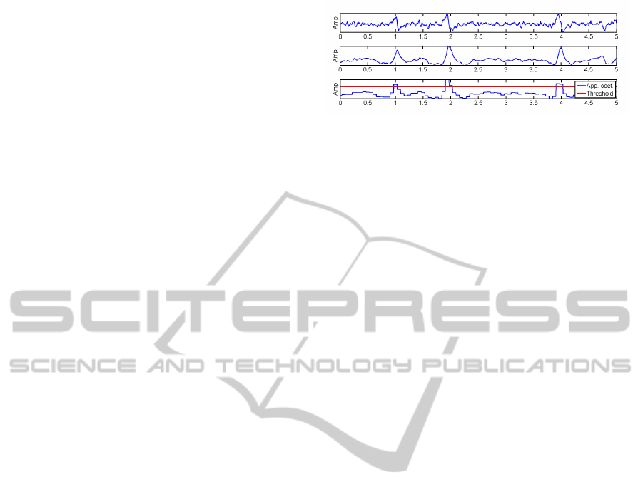
Figure 1: Illustration of method for component selection.

features are extracted from these components. Then,

the drowsiness detection is performed. Two methods

have been developed: one based on linear regression

and one on fuzzy detection. Finally, both methods

are validated by comparing the results with the KSS-

rating.

3.1 Component Decomposition

A Blind Source Separation method (BSS), BSS-CCA,

is used to decompose the signal in different compo-

nents arising from different sources:

X(t) = A ·s(t) (1)

X(t) is the measured EEG signal, s(t) are the different

sources and A is a mixing matrix that represents the

distribution of the different sources over all channels.

BSS-CCA will generate components that are mutu-

ally uncorrelated but with maximal temporal correla-

tion within each component. The complete algorithm

is described by De Clercq et al. (De Clercq et al.,

2006).

The signal is ﬁrst divided in subsequent epochs of

1 second. One second is experimentally determined to

be the optimal window length for this dataset. BSS-

CCA decomposes this epoch in components. If the

EEG signal has n channels, the result will be n com-

ponents.

3.2 Component Selection

The identiﬁcation of the EOG components is done

using a wavelet-based method, based on Krishnaveni

et al. (Krishnaveni et al., 2006). Figure 1 illustrates

the different steps.

First, each component is scaled with a coefﬁcient

= A(1, i) (2)

A is the mixing matrix from Equation (1), i is the in-

dex of the components. The ﬁrst row of the mixing

matrix corresponds to electrode Fp1. Since eye blinks

are best visible on the signal of this electrode, the am-

plitude of the artifact-components will enlarge, lead-

ing to easier detection. This can be seen on Figure 1:

the ﬁrst row is an epoch containing three eye blinks

BIOSIGNALS2014-InternationalConferenceonBio-inspiredSystemsandSignalProcessing

206

and the second row is one of the scaled components,

where the actual eye blinks are more clearly visible.

Each component is then decomposed with the Haar

wavelet up to 4 levels. The Haar wavelet is used since

Salwani and Jasny show that it gives the best results

in detecting ocular artefacts compared to other mother

wavelets (Salwani and Jasmy, 2005) . The reconstruc-

tion of the approximation coefﬁcients results in a step

function with a rising edge when the eye closes and a

falling edge when the eye opens, as is shown on the

third row of Figure 1. When there is no ocular artifact

present in the component, the approximation coefﬁ-

cients will have low values. The artifact components

are then identiﬁed by comparing the maximal approx-

imation coefﬁcient with a threshold of 80. If the max-

imum is larger than 80, the component is identiﬁed as

an EOG component. The value of 80 has been deter-

mined experimentally. When the epoch contains no

artifacts, the component with the highest approxima-

tion coefﬁcient is selected. This way, for each epoch

j, a new signal X

EOG

(t) is constructed:

EOG, j

(t) =

∑

i=1

(1, i) · s

i, j

(t) ∀ j (3)

In this equation, j is the index of the epoch, A

and

are respectively the mixing matrix and components

found in epoch j, i is the index of the component and

k are the number of components identiﬁed as EOG.

When the signals for all epochs are concatenated,

they form a signal with the same length as the orig-

inal EEG signal but with only one row. The newly

formed signal, from now on referred to as ’artifact

signal’, contains all artifacts found by BSS-CCA and

only minimal EEG information. It is thus ideal for the

derivation of different eye blink features.

3.3 Feature Calculation

First, the time instance when the artifact is at peak

amplitude is detected using the wavelet-based method

described in Section 3.2. The approximation coefﬁ-

cients are now compared with a threshold to detect

the individual eye blinks. Now, the threshold is deter-

mined for each subject individually to make detection

more accurate. The actual moment of the peak ampli-

tude is then found by looking for a local maximum in

the artifact signal 0.15 s around the detected blink.

Four points are detected for each eye blink, which

are indicated on Figure 2: the onset (red) and end

(blue) of the eye blink, the half-rise time (green) and

the half-fall time (orange). First, a moving average ﬁl-

ter with length ten samples smooths the artifact signal.

The ﬁrst derivative of the smoothed signal consists of

a part larger than zero followed by a part smaller than

Figure 2: Eye blink with detected points (Svensson, 2004).

zero, corresponding to the rising and falling ﬂank of

the eye blink. The onset and end are then found by

looking for zero-crossings in the derivative.

For each eyeblink, 16 features are now derived

from these values that can be grouped in three groups:

amplitude features, time features and velocity fea-

tures. The different features and their calculation are

listed in Table 1. During the experiment, the subject

only had to score his drowsiness on the KSS-scale

once every ﬁve minutes. Therefore, all eyeblinks in

each ﬁve minute interval are grouped together and two

values for each feature are calculated: the mean value

and standard deviation over a ﬁve minute interval.

This means that in the end there are 32 features.

3.4 Drowsiness Detection

Training data are used to determine which features are

affected by drowsiness and to set the different param-

eters needed for the prediction. A sufﬁcient amount of

training data is needed since the training data need to

contain enough variation in drowsiness levels. In this

case, the data of the second drive are used as training

data, the data of the third drive as test data.

The calculation of all 32 features is done for the

training data and Pearson’s product-moment correla-

tion coefﬁcient between the KSS-rating and each fea-

ture is then computed (Fenton and Neil, 2012). The

signiﬁcance of the correlation coefﬁcient is measured

by its p-value. When p is close to zero, there is sig-

niﬁcant correlation. The p-values of all correlation

coefﬁcients are calculated and sorted in increasing or-

der. Both methods use maximally the m features with

a p-value smaller than 0.2. Typically, p-values of 0.01

or 0.05 are used, but this value was increased to assure

that at least one feature is chosen so drowsiness can

be predicted. It is also possible to use less features,

in that case the n features with the lowest p-values are

selected.

3.4.1 Detection based on Linear Regression

Hargutt and Kruger show that there is a linear

relationship between various EOG parameters and

AdvancedEEGProcessingfortheDetectionofDrowsinessinDrivers

207

Table 1: EOG features and their calculation.

Group Feature Calculation

Amplitude

Peak amplitude Peak amplitude

Rise value Peak amplitude – onset amplitude

Fall value Peak amplitude – end amplitude

Onset difference Onset amplitude – end amplitude

Time

Total length End time – onset time

Rise length Peak time – onset time

Half-rise length Peak time – half-rise time

Half-fall length Half-fall time – peak time

Fall length End time – peak time

Half length Half-fall time – half-rise time

Time between two blinks

∆(peaktime)

∆t

Velocity

Rise velocity

Rise value

Rise length

Half-rise velocity

0.5∗Rise value

Hal f −rise length

Fall velocity

Fall value

Fall length

Half-fall velocity

0.5∗Fall value

Hal f − f all length

Total velocity

Rise value

Total length

drowsiness stages (Hargutt and Kruger, 2001). For

each of the selected features, this linear relationship

between the feature and the KSS rating is modeled by

ﬁtting them with a polynomial of degree 1:

KSS = a

· f eature + b

(4)

The process of detecting the eye blinks and calcu-

lating the features is now repeated for the test data.

Only the features that had signiﬁcant correlation in

the training data are calculated. The drowsiness is

then predicted by using linear regression to predict

the drowsiness based on each feature and taking the

average over all predictions:

KSS =

∑

i=1

KSS

(5)

∑

i=1

· f eature

+ b

(6)

i is the feature’s index and n is the number of fea-

tures that are used to predict the drowsiness, which

can range from 1 to m. Increasing n will increase the

number of features used, but each extra feature will

have a less strong correlation with the KSS rating than

the previous features.

3.4.2 Fuzzy Detection

The second method is based on a paper by Picot et al.

(Picot et al., 2011). For each feature that is used, two

parameters a and b are calculated:

a = µ

+ 0.25µ

(7)

b = µ

− 0.25µ

(8)

where i is the index of the feature and µ

the mean

value of feature i in the training data. The feature

calculation is repeated for the test data, and the cal-

culated features are converted to fuzzy indicators: a

number between 0 and 1 that indicates the drowsy

state. When this number is closer to one, the drowsi-

ness level will be higher. When the correlation be-

tween the feature and the KSS rating is positive, the

fuzzy drowsiness indicator is calculated by:

D( f

) =











0, if f

≤ a

−a

b−a

, if a ≤ f

≤ b

1 if f

≥ b

(9)

When the correlation is negative, Equation (9) be-

comes

D( f

) =











1, if f

≤ a

−b

b−a

, if a ≤ f

≤ b

0 if f

≥ b

(10)

In both equations (9) and (10), D is the drowsiness in-

dicator, i the index of the feature and f

the value of

feature i. Finally, the mean of the drowsiness indica-

tors is taken and converted to a number between one

and nine:

KSS = 8 · (

∑

i=1

) + 1 (11)

n is again the number of features used to predict the

drowsiness, which can be varied to include more or

less features.

3.5 Validation

Finally, the prediction results are compared with the

KSS rating given by the subjects to examine the qual-

BIOSIGNALS2014-InternationalConferenceonBio-inspiredSystemsandSignalProcessing

208

ity of the prediction. The comparison can be pre-

sented by constructing a confusion matrix. The values

on the diagonal are the most important values, since

they represent a perfect prediction. However, since

KSS is a scale with nine gradations, results where

the prediction differs one value from the true rating

can also be considered good results. Therefore, from

now on the distinction will be made between perfect

results (e.g. the predicted value is equal to the real

value) and good results (e.g. the difference between

the predicted and true value is one).

4 RESULTS

The eye blinks present in the signal are ﬁrst counted

manually and the result is compared with the num-

ber of eye blinks detected by the methods described

in Section 3. The developed methods detect in total

85.7 ± 8.1% of all eye blinks. The different features

and their correlation with the KSS rating are then cal-

culated. Features for which the correlation coefﬁcient

is small enough are used for drowsiness detection.

The ten features that are most often used to detect

drowsiness are listed in Table 2.

Table 2: Features included in most subsets.

Feature %

Mean half-rise speed 89.4

Mean rise speed 84.22

Mean fall value 78.9

Std half-fall length 78.9

Mean half-fall speed 78.9

Mean rise value 73.6

Mean half-rise length 73.6

Mean rise-length 73.6

Mean peak amplitude 73.6

Std total length 73.6

The ﬁrst column is the name of the feature and the

second column the percentage of subsets that includes

the feature. When a feature is included in a lot of sub-

sets, it means that the correlation between the feature

and the KSS rating is signiﬁcant for a lot of subjects.

The majority of the most frequently included features

are calculated as the mean value over a ﬁve-minute

interval. Only two features are the standard deviation

over a ﬁve-minute interval.

4.1 Method 1: Linear Regression

Figure 3 (a) shows the results for the drowsiness de-

tection using the ﬁrst method for one subject. The

predicted values are shown in red, the true values in

Figure 3: Results for drowsiness detection using method 1

(left) and method 2 (right).

blue. One thing is immediately clear: the predicted

values and true values have the same trend over time,

but there appears to be a constant difference of four

between the red and blue values. This difference,

or bias, is observed in almost all results. If the bias

is added to the predicted values, the results improve

tremendously: in the example from Figure 3 orig-

inally only 12% of the results were predicted well

(meaning a difference of one between the predicted

and the true value) and none of the values were pre-

dicted perfectly. If a bias of four is added, 75% of the

results are good and 54% of the results are perfect.

For each subject, the bias is determined visually and

added to the predicted values.

In Equation (6), n, the number of features used

to predict drowsiness can be varied. In Table 3 (a)

the average percentage of good results is shown for

different numbers of features used.

Table 3: Effect of number of features of results of (a) linear

regression and (b) fuzzy detection for one subject.

(a) Linear regression

Number % good

1 75.4

2 37.9

3 25.6

4 14.7

5 9.13

(b) Fuzzy detection

Number % good

1 71.4

2 68.1

3 63.4

4 61.8

5 60

The best results are obtained using only one fea-

ture. The accuracy decreases consistently with rising

n. Therefore, the number of features is ﬁxed at one

and the complete dataset is processed likewise. The

confusion matrix is shown in Table 4, the sum of the

good and perfect results is shown at the end of each

row.

The drowsiness prediction works well for large

KSS values. When the true value is one or two how-

ever, the majority of the predictions are wrong.

The results for individual subjects are good as

well. On average, 72 ± 18% of the predictions are

good. The percentage of perfect results is a lot lower:

29 ± 11%

AdvancedEEGProcessingfortheDetectionofDrowsinessinDrivers

209

Table 4: Confusion matrix for linear regression expressed in percentages.

Predicted value

1 2 3 4 5 6 7 8 9

1 0 1.85 22.22 25.92 25.92 14.81 7.40 1.85 0 1.85

2 0 8.33 8.33 58.33 25 0 0 0 0 16.66

3 0 3.22 35.48 45.16 0 3.22 6.45 3.22 3.22 83.86

4 0 0 24.50 32.35 19.60 8.82 2.94 5.88 5.88 76.45

True 5 0 0.76 6.87 22.13 22.13 26.71 14.50 2.29 4.58 70.97

value 6 1.76 1.76 4.42 7.07 13.27 26.54 38.05 6.19 0.88 77.86

7 2.87 2.15 0.71 1.43 7.19 12.94 33.09 30.93 8.63 76.96

8 0.69 1.38 1.38 1.38 3.47 4.86 25 29.86 31.94 86.8

9 3.33 1.11 1.11 2.22 6.66 14.44 10 11.11 50 61.11

4.2 Method 2: Fuzzy Detection

The second method again has a bias, as can be seen on

Figure 3(b), although the bias is smaller. Table 3(b)

shows that using one feature also gives the best result

in this case.

Table 5 shows the confusion matrix.

The predictions for a KSS rating of one are not

good: only 6.45% is predicted well. the results for

the other values are a lot better, the majority of predic-

tions differ maximum one value from the true rating.

After examining the results of all subjects, 34 ± 12%

of all predictions are perfect and 65±12.2% are good.

5 DISCUSSION

In this paper, drowsiness is detected based on the arti-

facts in the EEG signal. Equation 3 constructs a new

signal containing all artifacts and a minimum of EEG

signal. The signal will be similar to the EOG signal,

measured by placing electrodes around the eye, since

the EOG signal also contains all EOG artifacts and

minimal EEG signal. It would therefore be possible

to use the described methods with electrodes placed

around the eye. The advantage would be a reduction

in the number of electrodes which would beneﬁt the

user friendliness. However, an advantage of using the

complete EEG signal is that it contains a lot more in-

formation than merely EOG artifacts. This informa-

tion can be either be used for other purposes (such as

stress or concentration monitoring) or can be incorpo-

rated in the drowsiness detection to make the results

more accurate. Since CCA can effectively remove

both ocular and muscle artifacts, further calculations

can immediately be done on the clean EEG signal.

This makes the detection of other drowsiness indica-

tions in the EEG signal easier, since they are often

missed when the signal quality is bad (Simon et al.,

2011). It would be very interesting to repeat the cal-

culations using less electrodes, to see if similar results

can be obtained. This would increase the practical us-

ability, while still recording EEG signals that can be

used for further drowsiness detection.

The optimal number of features to detect drowsi-

ness is shown to be one. In one way, this could be

expected since the features are sorted based on the

signiﬁcance of their correlation. The feature with the

strongest correlation gives the best results. Adding

next important features didn’t increase the detection

performance, even in the case when the ﬁrst predic-

tion was incorrect. This indicates that the correlation

of the ﬁrst feature is a lot more signiﬁcant than the

other features.

Table 2 shows ”the most popular” features for

each set of training data. Mean speed and mean half-

rise speed are clearly two key features; they are in-

cluded in the majority of the subsets. First it has to be

noted that it is very probable that the rise speed and

half-rise speed are very correlated with each other. If

the speed of the total eye opening increases, it is ex-

pected that the speed at which half the eye opens in-

creases as well. Therefore it might be useful to ﬁrst

reduce the number of features using principal compo-

nent analysis. PCA can be used to convert a set of

possibly correlated variables to a set of linearly un-

correlated variables (Abdi and Williams, 2010). Sec-

ond, it is curious that the correlation of the rise speed

decreases most with increasing drowsiness. (Yue,

2011), (Svensson, 2004) and (Borghini et al., 2012)

all state that eye parameters such as blink duration

and frequency are inﬂuenced most by drowsiness, but

no one of them names velocity as an important pa-

rameter. The reason for this difference might lie in

the nature of the experiment. During the experiment,

the participants had to look at a screen for longer than

three hours. (Rosenﬁeld, 2011) demonstrates that this

may reduce the blink rate and cause Computer Vision

Syndrome, leading to dry and irritated eyes, which

may again inﬂuence eye blink behaviour. It is thus

BIOSIGNALS2014-InternationalConferenceonBio-inspiredSystemsandSignalProcessing

210

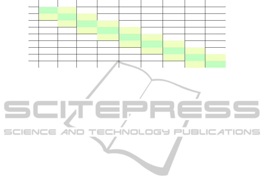
Table 5: Confusion matrix for fuzzy detection expressed in percentages.

Predicted value

1 2 3 4 5 6 7 8 9

1 0 6.45 9.67 25.8 12.9 16.12 19.35 3.22 6.45 6.45

2 0 6.25 25 50 6.25 6.25 6.25 0 0 31.25

3 0 1.47 29.41 32.35 23.52 7.35 2.94 1.47 1.47 63.23

4 0 .99 0.99 16.83 31.68 23.76 14.85 3.96 2.97 3.96 72.27

True 5 0 2.06 3.09 19.58 21.64 18.55 14.43 11.34 9.27 59.77

value 6 2.43 1.62 9.75 7.31 12.19 30.89 22.76 10.56 2.43 65.84

7 3.61 1.2 1.8 4.81 8.43 13.85 41.56 16.26 8.43 71.76

8 0.84 0.84 1.68 2.52 4.2 6.72 22.68 42.01 18.48 83.17

9 5.26 0 3.15 2.10 1.05 7.36 10.52 8.42 62.10 70.52

probable that in a natural environment (e.g. while

driving a real car instead of a driving simulator) other

features will be more important. Since using one fea-

ture gives the best prediction results and mean speed

and mean half-rise speed are clearly features that of-

ten have signiﬁcant correlation with the drowsiness

level, it would be possible to only calculate one of

both features.

Figure 3 shows that there is a difference between

the drowsiness level predicted and the true drowsiness

level. The bias is different for each subject. There

could be two reasons why there is a bias present. First,

the subjects do not rate their drowsiness consistently.

They for example think they are less tired than they

actually are. Since the subjects rate their drowsiness

after a questionnaire is shown on a screen, it is pos-

sible that the appearance of this questionnaire inﬂu-

ences the perceived drowsiness. If that is the case,

the questionnaire arouses the subject for a short time,

effectively decreasing the drowsiness rating. There-

fore, it would be interesting to obtain a more objec-

tive drowsiness rating by analyzing video recordings

or the driving behaviour of the subjects. Second, the

coefﬁcients of the polynomial that is ﬁtted to the train-

ing data might not be entirely correct. This may be ex-

plained by the fact that there are not many data avail-

able for low KSS values.

The second reason is obviously not relevant for

explaining the offset in the second method since no

linear ﬁt is used. However, there is also a bias no-

ticed in the results of the second method, although the

bias is smaller than in the results of the ﬁrst method.

Therefore, it is suspected that both reasons apply in

this case.

Finally, the results of both methods can be con-

sidered good, also when compared with other similar

methods. Svensson (Svensson, 2004) detects drowsi-

ness based on changes in blink behaviour and uses a

four graded scale. There, a correspondence with KSS

values of 70% is obtained. Picot et al. (Picot et al.,

2011) obtain an accuracy of 82% when distinguishing

between drowsy and not-drowsy, making the classiﬁ-

cation signiﬁcantly easier.

It is not easy to choose the best method among the

two tested here, since they both have their strengths

and weaknesses. If the two confusion matrices are

compared, it is clear that the method based on fuzzy

detection gives more perfect results and the linear

regression-based method gives more good results.

The differences are however small. They also show

that the fuzzy detection performs better for small KSS

values (although the result for KSS = 1 is still not

good). However, since the aim is detecting drowsi-

ness, large values are more important. Even more,

since drowsiness varies gradually, a small difference

in the true and predicted values is not very important.

Therefore, in most applications the linear-regression

based method would be preferred. However, when

perfect classiﬁcations need to be obtained, one would

probably start with fuzzy detection. In that case, the

method would have to be adjusted to improve the ac-

curacy.

6 CONCLUSIONS

The methods described in this paper are ways of de-

tecting drowsiness based on EOG artifacts present in

the EEG signal. They work semi-automatic: both the

threshold to detect eyeblinks and the bias are deter-

mined individually. The results of the methods are

good when perfect accuracy is not required. On av-

erage 70% of the predictions differ at most one value

from the KSS rating given by the subject. In applica-

tions when perfect accuracy is required however, the

methods should be improved or combined to give bet-

ter results. The results of the drowsiness detection

could be improved by extending the developed meth-

ods. It is possible to incorporate more information

extracted from the EEG in the methods. This way, the

accuracy and more speciﬁcally the number of perfect

results would be increased.

AdvancedEEGProcessingfortheDetectionofDrowsinessinDrivers

211

If the methods were to be used in real-life appli-

cations, they need to be used in real-time. Therefore,

the methods would have to be adapted. It would for

example be possible to calculate the features in a slid-

ing window, hereby giving a continuous prediction.

The thresholds for eye blink detection, which are now

deﬁned manually, can be ﬁxed during a test drive. To

increase the practical usability, the number of elec-

trodes should be decreased, since it is virtually impos-

sible to equip drivers with a full EEG cap. Finally, to

reduce the computational load, it can be researched if

the method gives good results when only calculating

one or two features, instead of calculating 32 features

and selecting one of them.

REFERENCES

A.A.A. Foundation (2010). Asleep at the wheel: The preva-

lence and impact of drowsy driving.

Abdi, H. and Williams, L. (2010). Principal component

analysis. Wiley Interdisciplinary Review: computa-

tional statistics, (2):433–459.

Borga, M. and Knutsson, H. (2001). A canonical ap-

proach to Blind Source Separation. Report LiU-

IMT-EX-0062 Department of Biomedical Engineer-

ing, Linkping University.

Borghini, G., Astolﬁ, L., Vecchiato, G., Mattia, D., and Ba-

biloni, F. (2012). Measuring neurphysiological signals

in aircraft pilots and car drivers for the assessment

of mental workload, fatigue and drowsiness. Neuro-

science and Biobehavioral Reviews, pages 45–57.

De Clercq, W., Vergult, A., Vanrumste, B., Van Paesschen,

W., and Van Huffel, S. (2006). Canonical Correla-

tion Analysis Applied to Remove Muscle Artifacts

From the Electroencephalogram. IEEE transactions

on Biomedical Engineering, 53(12):2583–2587.

Fenton, N. and Neil, M. (2012). Correlation coefﬁcient and

p-values: what they are and why you need to be wary

of them. In Risk assessment and Decision Analysis

with Bayesian Networks. CRC Press.

Geetha, G. and Geethalakshmi, S. (2011). Scrutinizing dif-

ferent techniques for artifact removal from EEG sig-

nals. International Journal of Engineering Science

and Technology, (1).

Hargutt, V. and Kruger, H. (2001). Eyelid movements and

their predictive value for fatigue stages. In Interna-

tional Conference on Trafﬁc and Transport Psychol-

ogy.

Homan, R. W., Herman, J., and Purdy, P. (1987). Cere-

bral location of international 10–20 system electrode

placement. Electroencephalography and clinical neu-

rophysiology, 66(4):376–382.

Hu, S. and Zheng, G. (2009). Driver drowsiness detection

with eyelid related parameters by support vector ma-

chine. Expert Systems with Applications, 36(4):7651–

7658.

Kaida, K., Takahasi, M., Akerstedt, T., Nakata, A., Otsuka,

Y., Haratani, T., and Fukasawa, K. (2006). Valida-

tion of the Karolinska sleepiness scale against perfor-

mance and EEG variables. Clinical Neurophysiology,

7(117):1574–1581.

Krishnaveni, V., Jayaraman, S., Aravind, S., Hariharasud-

han, V., and Ramadoss, K. (2006). Automatic Iden-

tiﬁcation and Removal of Ocular Artifacts from EEG

using Wavelet Transform. Measurement science re-

view, 6(2):45–57.

Picot, A., Charbonnier, S., and Caplier, A. (2011). EOG-

based drowsiness detection: Comparison between

a fuzzy system and two supervised learning classi-

ﬁers. Preprints of the 18th IFAC World Congress,

18:14283–14288.

Reyner, L. and Horne, J. (1998). Falling asleep whilst driv-

ing: are drivers aware of prior sleepiness? Int J Legal

Med, 3(111):120–123.

Rosenﬁeld, M. (2011). Computer vision syndrome: a re-

view of ocular causes and potential treatments. Oph-

thalmic and Physiological Optics, 31(5):502–515.

Salwani, M. and Jasmy, Y. (2005). Comparison of few

wavelets to ﬁlter ocular artifacts in eeg using lifting

wavelet transform. In TENCON 2005 2005 IEEE Re-

gion 10, pages 1–6. IEEE.

Simon, M., Schmidt, E. A., Kincses, W. E., Fritzsche, M.,

Bruns, A., Aufmuth, C., Bogdan, M., Rosenstiel, W.,

and Schrauf, M. (2011). Eeg alpha spindle measures

as indicators of driver fatigue under real trafﬁc condi-

tions. Clinical Neurophysiology, 122(6):1168–1178.

Svensson, U. (2004). Blink behaviour based drowsiness de-

tecion - method development and validation. Master’s

thesis, University of Link

oping.

Vergult, A., De Clercq, W., Palmini, A., Vanrumste, B.,

Dupont, P., Van Huffel, S., and Van Paesschen, W.

(2007). Improving the Interpretation of Ictal Scalp

EEG: BSS-CCA algorithm for muscle artifact re-

moval. Epilepsia, 48(5):950–958.

Verwey, W. B. and Zaidel, D. M. (2000). Predicting drowsi-

ness accidents from personal attributes, eye blinks and

ongoing driving behaviour. Personality and Individual

Differences, 28(1):123–142.

Vuckovic, A., Radivojevic, V., Chen, A. C., and Popovic,

D. (2002). Automatic recognition of alertness and

drowsiness from eeg by an artiﬁcial neural network.

Medical Engineering & Physics, 24(5):349–360.

Yue, C. (2011). EOG signals in drowsiness research. Mas-

ter’s thesis, University of Link

oping.

BIOSIGNALS2014-InternationalConferenceonBio-inspiredSystemsandSignalProcessing

212