
On the Robustness of the Biological Correlation Network Model
Kathryn M. Dempsey and Hesham H. Ali
College of Information Science & Technology, University of Nebraska at Omaha, Omaha, NE, 68182, U.S.A.
Keywords: Correlation Networks, Network Stability.
Abstract: Recent progress in high-throughput technology has resulted in a significant data overload. Determining how
to obtain valuable knowledge from such massive raw data has become one of the most challenging issues in
biomedical research. As a result, bioinformatics researchers continue to look for advanced data analysis
tools to analysis and mine the available data. Correlation network models obtained from various biological
assays, such as those measuring gene expression levels, are a powerful method for representing correlated
expression. Although correlation does not always imply causation, the correlation network has been shown
to be effective in identifying elements of interest in various bioinformatics applications. While these models
have found success, little to no investigation has been made into the robustness of relationships in the
correlation network with regard to vulnerability of the model according to manipulation of sample values.
Particularly, reservations about the correlation network model stem from a lack of testing on the reliability
of the model. In this work, we probe the robustness of the model by manipulating samples to create six
different expression networks and find a slight inverse relationship between sample count and network
size/density. When samples are iteratively removed during model creation, the results suggest that network
edges may or may not remain within the statistical parameters of the model, suggesting that there is room
for improvement in the filtering of these networks. A cursory investigation into a secondary robustness
threshold using these measures confirms the existence of a positive relationship between sample size and
edge robustness. This work represents an important step toward better understanding of the critical noise
versus signal issue in the correlation network model.
1 INTRODUCTION
The correlation network model has been used for
data modelling in multiple research studies
(Halappanavar et al., 2012); (Dempsey et al., 2011);
(Song et al., 2012); (Opgen-Rhein and Strimmer,
2007); (Horvath and Dong, 2008); (Verbitsky et al.,
2004); (Bender et al., 2008) that harness the power
of a network model to identify biological function.
While these studies have found great success in
identifying biological function (high degree nodes
can reflect essentiality (Halappanavar et al., 2012);
(Dempsey et al., 2011), clusters of nodes can
regulate or execute common cellular mechanisms
1,2
,
graph theoretic filters can remove noise from the
model while enhancing signal (Halappanavar et al.,
2012); (Dempsey et al., 2011); (Song et al., 2012);
(Opgen-Rhein and Strimmer, 2007)), the robustness
of the correlations used in the network model have
not been thoroughly examined.
Briefly, the correlation network model is
described as thus: a node represents a gene product
or probe from a high-throughput assay, such as a
DNA microarray or RNA-seq experiment. Each
experiment has some number of samples, n. For
each pair of genes or probes in the dataset, some
measure of correlation is applied. This correlation
assumes that there are at least three samples for each
gene/probe, and that none of the sample expression
values are missing, otherwise the correlation cannot
be performed for that pair. In cases where sample
size is small or experimental results are poor, a
majority of correlations may be rendered invalid, but
with improvement in current technologies this
becomes a much smaller issue.
For each pairwise comparison, a correlation
measure is used. Typically, this is the Pearson
correlation coefficient (which measure linear
relationships), but it can also include partial
correlation (where statistically calculated random
samples are not used in the correlation), Spearman
correlation (measuring relationships that are non-
linear using some function f), or other statistical
measures such as mutual information (measures the
186
M. Dempsey K. and H. Ali H..
On the Robustness of the Biological Correlation Network Model.
DOI: 10.5220/0004805801860195
In Proceedings of the International Conference on Bioinformatics Models, Methods and Algorithms (BIOINFORMATICS-2014), pages 186-195
ISBN: 978-989-758-012-3
Copyright
c
2014 SCITEPRESS (Science and Technology Publications, Lda.)

dependence of behaviour of one variable based on
another’s behaviour). After the correlation is
computed, some hypothesis testing is done to filter
out only significant correlations. In addition to
significance filtering, filtering via correlation
threshold is typically performed to reduce network
size and remove non-meaningful correlations (such
as those around 0.00).
There are two main ways to filter a network:
hard thresholding or soft thresholding. Hard
thresholding removes edges based on a firm cut-off
value; typically this value falls between the ranges
of -1.00 ≤ ρ ≤ -0.70 and 0.70 ≤ ρ ≤ 1.00. This
threshold is typically chosen as it captures only
relationships that are descriptive of the behaviour of
two genes. For example, a correlation of 0.70 has a
coefficient of determination (R
2
which is equivalent
to ρ
2
) of 49%, meaning that if the correlation reflects
a true relationship, 49% of a given gene’s behaviour
can be attributed to the other gene, and vice versa.
Soft thresholding, popularized by Horvath and
Dong (2008) (called WGCNA), involves identifying
the threshold at which the network exhibits scale-
free properties which some particular networks are
expected to have, and extracting the subnetwork of
the original network such that the filtered network is
scale-free. Thus, comparing two sets of expression
data from the same model and cell line but under
different environmental conditions might involve
using different correlation values based on the soft
thresholding approach.
While many studies have used iterations of the
correlation network model with success, few studies
in network systems in biology have delved into the
robustness of correlations, and how that might affect
network structure. For example, if a sample is
removed from the network, does the correlation that
results remain the same value or does it change
significantly? The correlation, if originally had
fallen within the proposed threshold and after
sample removal failed to fall within the threshold,
might not be representative of a true relationship in
the data. This begs the question: How many samples
are sufficient to assume a robust network? These and
other questions, if answered, can lead to insights
about how to remove noise from a correlation
network, and which relationships can be trusted,
without having to integrate extraneous biological
information. The novelty of this work lies in the lack
of understanding of the stability or by contrast,
vulnerability of the correlation network model.
While correlation does not imply causative
relationship, the measure is still able to capture those
relationships that are causative; in capturing
everything the measure is prone to noise. This
research investigates the possibility of using the
strength of correlation to remove some of that noise
and also can be used as evidence to suggest the
beginning of data-driven experimental studies.
Bioinformatics deals largely with publicly available
data; however, the results of the research here
suggest that we can improve the requirements of
those studies (i.e. increasing sample number) for use
in systems biology.
2 METHODS
Briefly, this work describes a cursory review of the
effect that single sample removal has on Pearson
correlation coefficient in a hard-thresholded setting.
To investigate, networks were created, thresholded,
and then samples were iteratively removed to
determine effect on correlation value.
2.1 Network Creation
Three datasets were chosen to highlight the
difference in sample number; all datasets had 9 or
less samples, reflecting the current state of high-
throughput technology where most expression
experiments contain samples, at minimum, in
triplicate. The datasets chosen were:
GSE5078 (Verbitsky et al., 2004) – Mus
musculus hippocampus mRNA, compared at 2
months and 15 months (Young and Middle-
Aged, respectively). Young dataset contains 9
samples and Middle-Aged dataset contains 9
samples.
GSE5140 (Bender et al., 2008) – Mus musculus
whole brain mRNA, compared at untreated and
creatine-treatment (Untreated and Creatine,
respectively). The Untreated dataset contains 6
samples, and the Creatine dataset contains 6
samples.
GSE46384 (Ikushima and Misaizu) –
Saccharomyces cerevisiae untreated or exposed
to 40g/l of isopropanol, (0IPA and 40IPA,
respectively). The 0IPA dataset contains 4
samples, and the 40IPA dataset contains 4
samples.
A threshold of 0.70 ≤ ρ ≤ 1.00 using Pearson
correlation coefficients was used to find correlated
expression relationships, and p-values were
computing using the Student’s T-test with a
threshold of p-value <0.0005 significance. Network
sizes for each are contained below in Table 1. The
GSE5140 networks were the largest by node count.
OntheRobustnessoftheBiologicalCorrelationNetworkModel
187
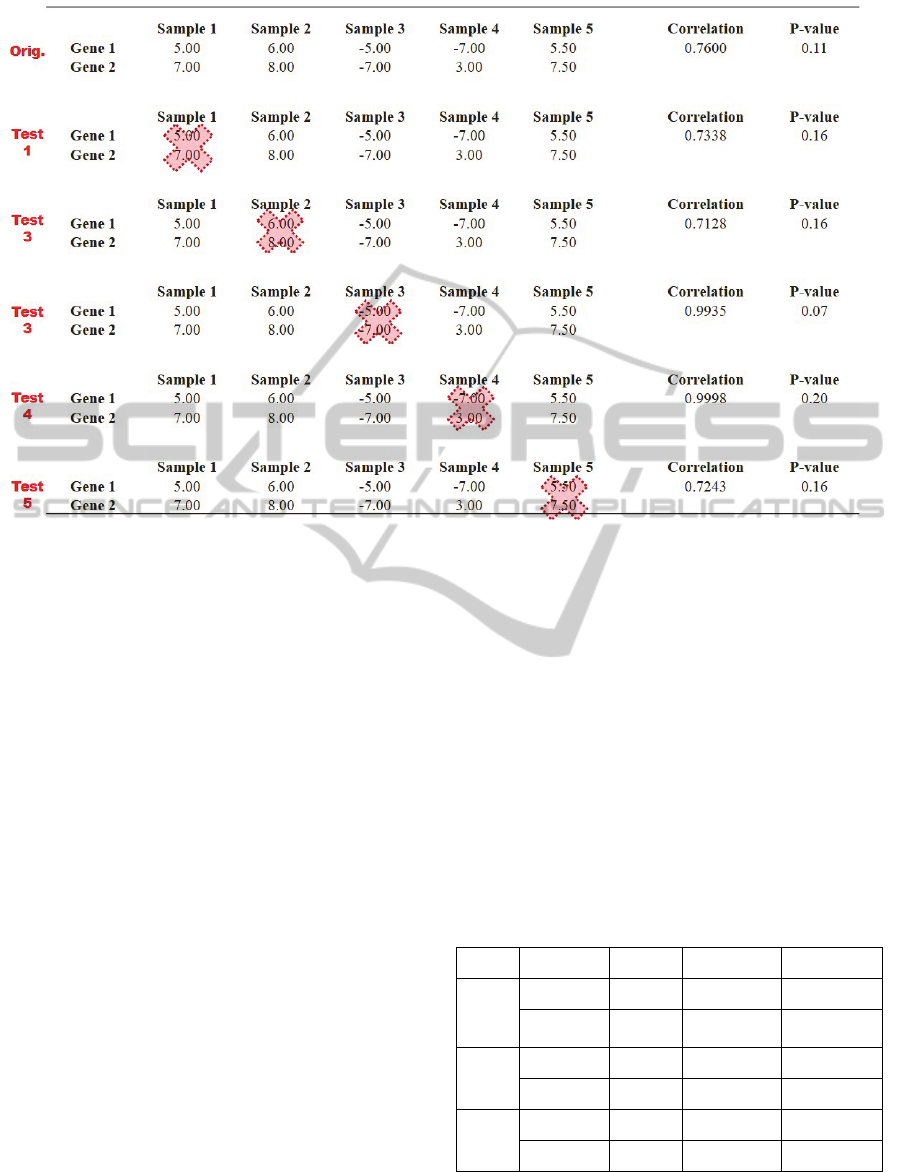
Figure 1: The process of removing samples to test robustness. The top rows (Orig) are the original correlation calculation
between five samples between Gene 1 and Gene 2. Samples 1-5 represent the expression values for each sample (can be
tissue, cell, etc.) In test 1, correlation is calculated between Samples 2-5, with Sample 1 removed for both Gene 1 and Gene
2. This results in a very slightly decreased correlation from the original (0.76 to 0.73) and a slightly increased p-value (0.11
to 0.16) meaning the correlation has less confidence. This occurs iteratively for each sample. If the correlation threshold
was 0.75 ≤ ρ ≤ 1.00 and a p-value <0.15, only the correlation for test 3 would pass the significance test, and its correlation
would pass the threshold test as well at 0.99. For this example, the PSC would be equal to 1/5 = 20%, the PTC would be 1/1
= 100%, and the PST would be 1/5, or 20%.
Despite being the smallest networks by node count,
the yeast GSE46384 networks were the densest at 8-
10% density. The GSE5078 networks were the
middle of the road in terms of node counts but had
the lowest density, meaning that these networks
were very sparse compared to total possible edges.
So, by density, there appears to be an inverse
relationship between sample size and resulting
network density. This is to be expected – using such
low sample counts to identify correlations means
that as more information becomes available, more
evidence is there to confirm or deny an actual
correlation. For example, it is easier to find a 100%
correlation of two probes with 3 samples than it is to
find a 100% correlation of two probes with 10
samples. (This does not, however, examine
significance). The GSE46384 networks had the
smallest amount of samples but the highest number
of edges per node on average. The GSE5140
network contained 6 samples and the middle of the
road density results; it should be noted that these
datasets contained the entire genome-wide set of
probes then available for mouse models. Finally, the
network with the most samples, GSE5078 at 9
samples results in the sparsest networks.
Table 1: Network edge counts. Column 1: GEO Series
number, Column 2: network name, Column 3: # nodes in
the thresholded/filtered network, Column 4: # edges in the
thresholded/filtered network, and Column 5: density of the
network, which is equal to Edge Count / (Node Count *
(Node Count -1)/2). We find that the lower the sample
count, the higher the density.
Dataset
Name Nodes Edges Density
GSE
5078
Young 12,390 923,794 1.2036%
Middle-
Aged
12,378 1,013,130 1.3226%
GSE
5140
Untreated 45,000 32,075,094 3.1679%
Creatine 45,004 33,349,407 3.2932%
GSE
46384
IPA0 6,301 1,616,710 8.1453%
IPA40 6,304 2,000,931 10.0716%
These types of results are typical of what is the
current standard in correlation networks. The more
samples there are, the more confident and strong the
BIOINFORMATICS2014-InternationalConferenceonBioinformaticsModels,MethodsandAlgorithms
188

correlation. Therefore, more noise can be removed
as sample number increases. We expect that the
GSE46384 network would be naturally filtered by
the addition of more samples, which would
strengthen relationships that actually exist via
strengthening correlations and their significance.
2.2 Robustness Testing
In datasets where sample size is small, there needs to
be some measure that limits the impact of errors or
outliers in the data. To accommodate potential error
and noise, we define robustness to determine the
reliability of the network model itself. Robustness of
a correlation is defined, in this particular study, as
the likelihood of a correlation to remain at or above
some threshold t after random sample removal. If a
correlation between two probes originally is 100%,
and falls to 90% after iterative sample removal, we
can say it is robust because it still falls within our
threshold of 0.70 ≤ ρ ≤ 1.00 (assuming both
correlations are also significant). If a correlation
between two probes originally is 100% and falls to
50% after individual sample removal, it would not
be considered a robust relationship. To test the
robustness of correlations according to sample
removal, a simple method was deduced. As per
normal network creation standards, networks were
made by pairwise computation of Pearson
Correlation between two probes and if the threshold
was met (0.70 ≤ ρ ≤ 1.00), hypothesis testing was
performed. If p-value was less than 0.0005, the edge
was considered for robustness testing.
To test robustness, samples were iteratively
removed from the gene pair vectors as shown in
Figure 1. For example, for two genes, each with five
samples, values of expression for sample 1 in both
probes were removed and correlation and
significance were calculated. If the correlation
between the manipulated probes was significant, the
correlation was kept. Next, sample 2 was removed,
and the correlation was again kept if it was
significant.
After all correlations and sample removal
correlations were reported, it was also necessary to
determine if the correlations found after sample
removal were also above or within the threshold
(within the bounds of the threshold = robust or
outside the bounds of the threshold = not robust).
To measure this, the following metrics were devised:
Percentage of Significant Correlations (PSC): the
number of significant correlations versus the
total possible significant correlations (sample
number). This measures the percentage of
significant correlations that result when a
sample is removed – the higher the better. 100%
is optimal.
Percentage of Threshold Correlations (PTC): the
number of correlations above some threshold t
versus the number of significant correlations.
This measures the percentage of significant
correlations that are above the threshold
required by the user. 100% again is optimal.
Percentage of Significant Threshold Correlations
(PST): the number of correlations that are
significant and above some threshold t versus the
total possible significant correlations. This
measures the percentage of significant
correlations that are above the threshold when
some sample is removed. 100% is optimal.
Also computed was the standard deviation for each
set of significant correlations. The following
equations (Equations 1-3, below) define how PSC,
PTC, and PST were computed, where n is equal to
sample number, t is the threshold given, s
corr
is equal
to the count of significant correlations, and t
corr
is
equal to the count of significant correlations above
the threshold t.
1:
2:
3:
Informally, PSC tells us the percentage of
correlations that remain statistically significant per
sample count, PTC tells us the percentage of
significant correlations that fall within the threshold,
and PST tells us the percentage of significant
correlations that fall within the threshold per sample
count.
2.3 Clustering and Enrichment
To test the biological function of normal versus
robustness tested networks, the top 5 clusters (based
on MCODE (Bader and Hogue, 2003) ranking) were
tested for biological function using the Gene Set
Enrichment Analysis tool via the Gene Trail (Backes
et al., 2007) tool (http://genetrail.bioinf.uni-sb.de/).
Clustering was performed using MCODE v.1.2
using the parameters: Degree cut-off of 10, Node
Score Cut-off of 0.2, Haircut set to True, K-core set
to 10, and Max Depth set to 10. The top 5 clusters
according to MCODE’s proprietary scoring method
(score = density * node count) and GSEA was
OntheRobustnessoftheBiologicalCorrelationNetworkModel
189

performed on node lists from each. GeneTrail
parameters used were: Only manually curated GO
annotations and a significance value of 0.05.
3 RESULTS
Comparing the scores of each network in terms of
PSC, PTC, and PST allows for characterization of
correlation robustness in a general way. In an ideal
network, all correlations are robust and sample size
is optimal for robustness. The goal of this research is
to address the robustness issue to determine the
ability of the correlation network model to represent
accurate biological information.
3.1 Non-optimal Correlations
To give a first insight into robustness, the original
network sizes were compared to network size when
correlations with no significant above-threshold
correlations are observed (Table 2). Here we
highlight the % Non-Robust Edges, which is the
percentage of edges in the original network that are
not robust, or those edges that do not fall within the
threshold t when a sample is removed. As sample
count increases, the level of non-robust edges
decreases.
Table 2: Insignificant, non-threshold robustness. Column
1: GEO Series #, Column 2: network name, Column 3:
edge # in the thresholded network, Column 4: edge # in
the thresholded network when non-robust, insignificant
edges are removed, Column 5: percentage of the original
network representing non-robust edges, 100% - (Robust
Edge Count/Original Edges). The number of removed
non-robust edges for any network is minimal, meaning
that significance of correlation at any sample size is trivial.
Dataset
Name
Original
Edges
Robust
Edge
Count
% Non-
Robust
Edges
GSE5078
Young 923,794 922,394 0.1515%
Middle-
Aged
1,013,130 1,011,586 0.1524%
GSE5140
Untreated 32,075,094 31,902,640 0.5377%
Creatine 33,349,407 33,121,663 0.6829%
GSE46384
IPA0 1,616,710 1,573,416 2.6779%
IPA40 2,000,931 1,930,502 3.5198%
However, the overall number of absolutely non-
robust edges overall is low, representing 0.1-3.5% of
the entire network edges. This means that the large
portion of edges in correlation networks are robust
to sample removal.
3.2 Variance in Robustness via PSC
To examine the distribution of robustness of
correlations, the PSC, PTC, and PST were calculated
for each correlation and mapped. These results for
PSC are contained in Figure 2. This figure highlights
the number of significant correlations versus the
sample number (x-axis) and the log of the count of
PSC scores at that point (y-axis). For example, the
green triangle in the topmost right corner of Figure 2
represents a PSC score of 100% with a very high log
(count), meaning that a large majority of the
correlations in the Untreated network are significant
when a sample is removed. All networks except for
the Untreated network find an increase in PSC from
0-50% and then a decrease or stabilization in PSC
from 50-100%. This indicates that there are many
relationships that become insignificant when
samples are removed; these correlations where
significance is lost become good candidates for
removal.
Figure 2: The PSC score distribution for all 6 networks. X-
axis: PSC score - The number of significant correlations
versus the sample number. Y-axis: The log of the count of
PSC scores. This measure shows per probe pairing how
many of the sample-removed correlations are significant.
I.e., if a probe pair has 10 samples and 5 of them are
significant correlations when a sample is removed, it will
have a 50% PSC score. The scores above suggest that
there is a large majority of correlations that lose their
significance when a sample is removed.
The results for PTC are contained in Figure 3.
This figure highlights the number of significant,
above threshold correlations when samples are
removed versus total sample size (X-axis) versus the
log of the count of PTC scores at that point.
Interestingly, in all but the Untreated and Creatine
networks, all networks find that if a correlation
remains significant after a sample is removed, it is
BIOINFORMATICS2014-InternationalConferenceonBioinformaticsModels,MethodsandAlgorithms
190
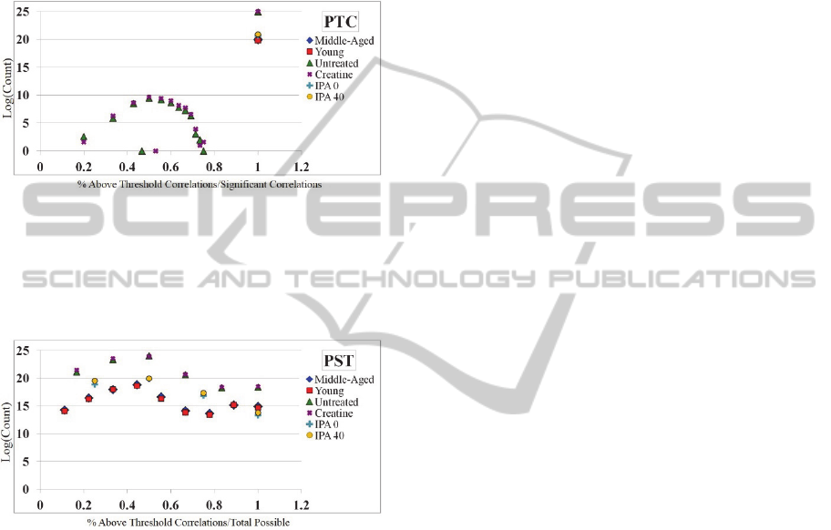
also within our given threshold t (100%). The
exception is in the Untreated and Creatine networks,
where there is again a distribution of scores from 20-
80% indicating that, for example, there is a portion
of relationships where sample removal results in a
correlation that is not within the given threshold t, or
not all sample-removed correlations that are
significant meet threshold requirements.
Figure 3: The PTC score distribution for all 6 networks.
X-axis: PTC score. Y-axis: The log of the count of PTC
scores. The results here indicate that for the majority of
networks, the number of significant correlations after
sample removal are also within threshold.
Figure 4: The PST score distribution for all 6 networks. X-
axis: PST score. Y-axis: The log of the count of PST
scores. The results here indicate that there is a distribution
of edges that do not meet the threshold and significance
requirements to be robust.
The results for PST are contained in Figure 4.
This figure highlights the number of significant,
above threshold correlations when samples are
removed versus significant sample-removed
correlations (X-axis) versus the log of the count of
PST scores at that point. The PST scores, perhaps
the most telling, reveal that there indeed exists a
distribution of correlations from approximately 10-
100%, where a large amount of edges relative to
network size find few significant above-threshold
correlations compared to significant correlations.
Interestingly, this number seems to drop off slightly
around 50%, and appears to stabilize or grow again.
Generally, this means that the large majority of
correlations within the network tend to be robust.
3.3 A Secondary Threshold?
How does this information impact the creation,
thresholding, and usage of the correlation network
model? Notoriously noisy (Reverter and Chan,
2008); (Song et al., 2012); (Opgen-Rhein amd
Strimmer, 20007), the correlation network model
tends to be underused due to the common reasoning
that “correlation does not imply causation;”
however, this does not mean that the measure does
not capture any information. Quite frankly, the
correlation measure captures all possible linear
relationship, but it is up to the user to determine if
those relationships are meaningful (Song et al.,
2012); (Opgen-Rhein and Strimmer, 2007). As such,
this research suggests that the correlation network
model may also benefit from having a secondary
threshold that is based on the robustness of the
correlation itself. While network size, density, and
absolutely non-robust edges seemed to be impacted
by sample size, the distribution of robust edges does
not appear to be significantly impacted by sample
size in our results above. Thus, it would appear that
correlations that are strong will become stronger by
the addition of samples, but will not become weaker
with single sample removal if the correlation is truly
representative of a biological co-regulated
relationship.
To begin to foray into the impact of a secondary
threshold, the natural dip in PSC, PTC, and PST
score distributions were used. This dip appears at or
around 50%, indicating that those correlations are at
least 50% likely to have a significant, within
threshold correlation after a sample is removed.
This 50% “secondary threshold” was used to
examine the effect of removing correlations where
robustness of PST is greater than or equal to 50%.
To clarify, consider two probes with 10 samples. If
each sample is individually removed and correlation
is calculated, the resulting correlation must be
significant and within the threshold t for at least
50% of the iterations (5 of the 10 correlations must
be significant and within t) for the edge to be
considered, otherwise it was thrown out. Removing
edges in this way reduces edge count; resulting
network sizes using this threshold are shown in
Table 3.
Using the secondary 50% PST threshold, we are
able to remove 40-80% of edges from the already
significance and thresholded original network.
Interestingly, the networks with the most samples
(Young and Middle-aged) found the highest edge
OntheRobustnessoftheBiologicalCorrelationNetworkModel
191

removal at 81.65% (Young) and 80.46% (Middle-
aged). This makes sense when you consider how
correlation is calculated – one would expect with 2
or 3 sample removal at a time, this edge reduction
percentage would decrease – but the magnitude of
edges that stand to be removed is very telling. This
means that, should the biological “signal” of the 2
nd
thresholded network be equal to or greater than the
biological signal of the original network, that we are
able to reduce the network size (and thus
computational time and load of analysis of the
model) drastically.
3.4 Preliminary Functional Analysis
To examine how the model may also benefit from
having a secondary threshold to reduce noise,
preliminary functional analysis was performed on
original and robustness thresholded networks to see
if it is able to remove noise that confounds
biological signal. Clustering using MCODE was
performed on both the Young original network and
the Young 2
nd
thresholded network, and the top 5
clusters were extracted (see Methods). After cluster
extraction, the nodes in each cluster were tested for
biological function using Gene Set Enrichment
Analysis. Only annotations with 4 or more observed
genes per cluster were considered. The results of this
enrichment on the Young network clusters are
shown in Figure 5. What was found is that for three
out of five of the original Young network clusters,
there were too many biological process annotations
to be relevant or helpful for decision support or to
determine the actual function (if any) of the cluster.
By comparison, each of the robustness network
filtered clusters contained 10 annotations or less.
The functions of these clusters need to be further
probed, but if the functions found in the robustness
thresholded clusters are found to be accurate, this
can be considered a major way to further remove
noise from the network and understand the functions
of the structures therein.
Top 10 Gene Ontology enrichment of clusters in
the middle-aged network clusters is shown in Figure
6. As in the young network, there were many
biological process tree annotations for original
clusters and fewer annotations in the robustness
filtered clusters. Future work will investigate the real
biological function of these clusters, and
additionally, the function of clusters in which
robustness is used as a filter. The results of this
approach might bring the speculation that robustness
filtered networks will return clusters with a more
refined biological function due to the fact that noise
(or correlations in which we are not confident) are
removed.
Table 3: Network edge reduction based on second
robustness threshold. Column 1: GEO Series number,
Column 2: network name, Column 3: # edges in the
thresholded/filtered network, Column 4: # edges in the
thresholded/filtered network after second thresholding,
and Column 5: percentage of edges that were removed
from the original network by this second threshold,
calculated as 100% - (2
nd
Threshold edges/Original
Edges). These results indicate that the more samples
present, the more edges can be removed, possibly because
sample size improves correlation confidence.
Dataset
Name Edges
2nd
Threshold
Edges
Edge
Reduction
GSE5078
Young 923,794 169,524 81.65%
Middle-
Aged
1,013,130 197,977 80.46%
GSE5140
Untreated 32,075,094 18,925,611 41.00%
Creatine 33,349,407 17,935,181 46.22%
GSE46384
IPA0 1,616,710 1,092,630 32.42%
IPA40 2,000,931 1,189,808 40.54%
4 DISCUSSION
Network theory in systems biology remains in
relative infancy, and the correlation network is no
exception to benchmarking necessity. While high
performance computing techniques have typically
been found to be needed for fast and thorough
analysis of network models, laboratories do not
always have access to these types of resources. The
results of these studies allow for the following
potential conclusions to be inferred from studies on
robustness the correlation network model; additional
testing will be necessary to confirm or deny their
existence:
1. Sample size and network density are inversely
linked – the smaller the sample count, the higher
the density.
2. Sample size and non-robustness are inversely
linked – the smaller the sample size, the more
absolutely non-robust edges a network will have.
3. Based on the distribution of robust correlations
compared to sample number, correlation
networks can be thresholded to further remove
noise due to coincidental expression patterns.
BIOINFORMATICS2014-InternationalConferenceonBioinformaticsModels,MethodsandAlgorithms
192

Figure 5: Top 10 Gene Ontology enrichment terms of GSE5078 Young network clusters, original (left) and robustness
thresholded (right). Column headings include GO Term/Annotation, GO ID, Obs., or Observed number of genes with that
term, P-value, and Up or Down enrichment (whether or not the cluster is over or under enriched for that term based upon
the yeast genome).
GOTERM GOID Obs. P‐Val
↑or↓
Term# GOTERM GOID Obs. P‐Val
↑or↓
macro.metabolicproc. GO:0043170 15 0.04 up 1 systemproc. GO:0003008 60.05 up
cellularmacro.metabolic
proc.
GO:0044260 14 0.02 up 2 reg.ofmolecularfunction GO:0065009 5 0.01 up
reg.ofmetabolicproc. GO:0019222 13 0.05 up 3 celladhesion GO:0007155 5 0.03 down
reg.ofprimarymetabolic
proc.
GO:0080090 13 0.05 up 4
positivereg.ofmetabolic
proc.
GO:0009893 5 0.03 up
negativereg.ofcellularproc. GO:0048523 12 0.03 up 5 biologicaladhesion GO:0022610 5 0.03 down
reg.ofmacro.metabolicproc. GO:0060255 10 0.02 up 6
positivereg.ofcatalytic
activity
GO:0043085 4 0.03 up
nucleicacidmetabolicproc. GO:0090304 10 0.02 up 7
positivereg.ofmolecular
function
GO:0044093 4 0.03 up
transcription GO:0006350 9 0.04 up 8 reg.ofcatalyticactivity GO:0050790 4 0.03 up
macro.biosyntheticproc. GO:0009059 9 0.04 up 9
reg.ofgeneexpression GO:0010468 9 0.04 up 10
plasmamembrane GO:0005886 13 0.04 up 1 molecular_function GO:0003674 450.03 up
membrane GO:0016020 13 0.04 up 2 proteinbinding GO:0005515 15 0.03 up
catalyticactivity GO:0003824 10 0.05 up 3 primarymetabolicproc. GO:0044238 12 0.03 down
signaling GO:0023052 8 0.02 up 4 macro.metabolicproc. GO:0043170 9 0.05down
signalingpway GO:0023033 7 0.03 up 5 reg.ofcatalyticactivity GO:0050790 5 0.01 down
cellsurfacerec.linkedsignal
pway
GO:0007166 6 0.05 up 6 reg.ofmolecularfunction GO:0065009 5 0.01 down
7
positivereg.ofcatalytic
activity
GO:0043085 4 0.02 down
8
positivereg.ofmolecular
function
GO:0044093 4 0.02 down
9 organellepart GO:0044422 4 0.04 down
10 intracellularorganellepart GO:0044446 4 0.04 down
developmentalproc. GO:0032502 56 0.02 up 1 multicellularorganism.proc. GO:0032501 15 0.04 down
multicellularorganism.dev. GO:0007275 50 0.03 up 2 developmentalproc. GO:0032502 13 0.02 down
systemdev. GO:0048731 46 0.04 up 3 anatom.struct.dev. GO:0048856 13 0.02 down
nucleus GO:0005634 39 0.03 up 4 multicellularorganism.dev. GO:000727512 0.04down
cellulardevelopmentalproc. GO:0048869 37 0.00 up 5 celldifferentiation GO:0030154 9 0.03 down
celldifferentiation GO:0030154 34 0.00 up 6 reg.ofbiologicalproc. GO:0050789 8 0.04 down
Metabolicpways 1100 23 0.05 down 7 reg.ofcellularproc. GO:0050794 8 0.04 down
celldev. GO:0048468 22 0.05 up 8 membrane GO:0016020 4 0.04 up
signalingproc. GO:0023046 22 0.05 up 9
signaltransmission GO:0023060 22 0.05 up 10
biologicalreg. GO:0065007 17 0.03 down 1 biological_proc. GO:0008150 290.02 up
reg.ofbiologicalproc. GO:0050789 15 0.03 down 2 metabolicproc. GO:0008152 16 0.03 up
reg.ofcellularproc. GO:0050794 13 0.05 down 3 macro.metabolicproc. GO:0043170 7 0.04 up
catalyticactivity GO:0003824 11 0.03 up 4 proteinbinding GO:0005515 6 0.03 up
cytoplasm GO:0005737 7 0.02 up 5 signaltransduction GO:0007165 6 0.03 up
hydrolaseactivity GO:0016787 7 0.02 up 6 hydrolaseactivity GO:0016787 5 0.03 up
cytoplasmicpart GO:0044444 6 0.04 up 7
negativereg.ofmetabolic
proc.
GO:0009892 4 0.03 up
8
negativereg.ofmacro.
metabolicproc.
GO:0010605 4 0.03 up
9 proteinmetabolicproc. GO:0019538 4 0.05 up
signaling GO:0023052 30 0.04 up 1
anatom.struct.
morphogenesis
GO:0009653 5 0.04 up
signalingpway GO:0023033 26 0.02 up 2
anatom.struct.formation‐
morphogenesis
GO:0048646 5 0.04 up
signalingproc. GO:0023046 19 0.01 up 3
signaltransmission GO:0023060 19 0.01 up 4
proteinmetabolicproc. GO:0019538 17 0.05 up 5
smallmoleculemetabolic
proc.
GO:0044281 16 0.04 up 6
cellproliferation GO:0008283 14 0.05 down 7
signaltransduction GO:0007165 13 0.01 up 8
reg.ofmolecularfunction GO:0065009 13 0.03 up 9
cellularproteinmetabolic
proc.
GO:0044267 13 0.04 up 10
ROBUST
Cluster1Cluster2Cluster3Cluster5 Cluster4
ORIGINAL
OntheRobustnessoftheBiologicalCorrelationNetworkModel
193

Figure 6: Top 10 Gene Ontology enrichment terms of GSE5078 Mid network clusters, original (left) and robustness
thresholded (right). Colum-n headings include GO Term/Annotation, GO ID, Obs., or Observed number of genes with that
term, P-value, and Up or Down enrichment (whether or not the cluster is over or under enriched for that term based upon
the yeast genome).
GOTERM GOID Obs. P‐Val ↑or↓ Term# GOTERM GOID Obs. P‐Val ↑or↓
homeostatic
p
roc. GO:0042592 12 0.05 u
p
1multicell.or
g
anism.
p
roc. GO:0032501 23 0.01 u
p
cell‐cellsi
g
nalin
g
GO:0007267 10 0.01 u
p
2
p
roteinbindin
g
GO:0005515 21 0.03 u
p
transferaseactivity GO:0016740 8 0.01 down 3
multicell.organism.
develo
p
ment
GO:0007275 16 0.05 up
inflammator
y
res
p
onse GO:0006954 7 0.04 down 4 s
y
stemdevelo
p
ment GO:0048731 16 0.05 u
p
s
y
na
p
tictransmission GO:0007268 6 0.01 u
p
5si
g
nalin
g
GO:0023052 11 0.04 u
p
transferaseactivit
y
GO:0016772 5 0.01 down 6 si
g
nalin
g
p
wa
y
GO:0023033 9 0.00 u
p
neuronalcellbod
y
GO:0043025 5 0.03 u
p
7or
g
anmor
p
h. GO:0009887 9 0.02 u
p
cellbod
y
GO:0044297 5 0.03 u
p
8si
g
naltransduction GO:0007165 9 0.03 u
p
solublefraction GO:0005625 5 0.04 down 9
cellsurfacereceptorlinked
si
g
nalin
g
p
wa
y
GO:0007166 8 0.01 up
MAPKsignalingpway 4010 4 0.03 down 10
positiveregulationofcell
p
roliferation
GO:0008284 5 0.02 up
cell GO:0005623 32 0.03 down 1 cellular_com
p
onent GO:0005575 51 0.05 u
p
cellpart GO:0044464 32 0.03 down 2
intracellularmem.‐bounded
or
g
anelle
GO:0043231 20 0.04 down
intracellularorganelle GO:0043229 20 0.04 down 3
macromoleculebiosynthetic
p
roc.
GO:0009059 15 0.03 down
anatomicalstructuremorph. GO:0009653 15 0.04 up 4
cellularnitrogencompound
metab.
p
roc.
GO:0034641 13 0.02 up
catal
y
ticactivit
y
GO:0003824 5 0.01 down 5 nucleus GO:0005634 13 0.04 down
positiveregulationofimmune
s
y
stem
p
roc.
GO:0002684 4 0.02 up 6 extracellularregionpart GO:0044421 12 0.05 down
re
g
ulationofimmuneres
p
onse GO:0050776 4 0.02 u
p
7nucleicacidmetab.
p
roc. GO:0006139 12 0.05 u
p
8 localization GO:0051179 11 0.02 down
9extracellulars
p
ace GO:0005615 10 0.04 down
10 si
g
nalin
g
p
wa
y
GO:0023033 10 0.02 down
cellular_com
p
onent GO:0005575 62 0.01 down 1 or
g
anmor
p
h. GO:0009887 9 0.01 down
biolo
g
ical_
p
roc. GO:0008150 59 0.02 down 2 celldifferentiation GO:0030154 9 0.01 down
p
roteinbindin
g
GO:0005515 30 0.02 down 3 cellulardevelo
p
mental
p
roc. GO:0048869 9 0.01 down
biologicalregulation GO:0065007 27 0.05 down 4
cellsurfacereceptorlinked
si
g
nalin
g
p
wa
y
GO:0007166 9 0.04 down
re
g
ulationofcellular
p
roc. GO:0050794 23 0.03 down 5 nervouss
y
stemdevelo
p
ment GO:0007399 8 0.01 down
multicell.or
g
anism.
p
roc. GO:0032501 23 0.05 down 6 tissuedevelo
p
ment GO:0009888 7 0.02 down
multicell.organism.
develo
p
ment
GO:0007275 17 0.04 down 7 locomotion GO:0040011 6 0.01 down
systemdevelopment GO:0048731 17 0.04 down 8
positiveregulationofmetab.
p
roc.
GO:0009893 6 0.02 down
macromoleculemetab.proc. GO:0043170 15 0.02 down 9
positiveregulationof
macromoleculemetab.
p
roc.
GO:0010604 6 0.02 down
positiveregulationofbiological
p
roc.
GO:0048518 15 0.02 down 10
positiveregulationofgene
ex
p
ression
GO:0010628 6 0.02 down
re
g
ulationofbiolo
g
ical
p
roc. GO:0050789 54 0.04 down 1 cellfraction GO:0000267 7 0.02 down
re
g
ulationofcellular
p
roc. GO:0050794 49 0.02 down 2 macromolecularcom
p
lex GO:0032991 7 0.04 u
p
nitro
g
enmetab.
p
roc. GO:0006807 24 0.01 down 3 cellulardevelo
p
mental
p
roc. GO:0048869 7 0.04 u
p
cellularnitro
g
enmetab.
p
roc. GO:0034641 24 0.01 down 4 catal
y
ticactivit
y
GO:0003824 5 0.01 down
bios
y
nthetic
p
roc. GO:0009058 23 0.03 down 5 solublefraction GO:0005625 5 0.02 down
nucleicacidmetab.
p
roc. GO:0006139 21 0.02 down 6 nervouss
y
stemdevelo
p
ment GO:0007399 4 0.03 u
p
g
eneex
p
ression GO:0010467 20 0.04 down 7 neuro
g
enesis GO:0022008 4 0.03 u
p
nucleicacidmetab.
p
roc. GO:0090304 20 0.04 down 8
g
enerationofneurons GO:0048699 4 0.03 u
p
re
g
ulationof
g
eneex
p
ression GO:0010468 19 0.04 down 9
regulationofmulticell.
or
g
anism.
p
roc.
GO:0051239 18 0.00 down 10
multicell.or
g
anism.
p
roc. GO:0032501 31 0.01 u
p
1bindin
g
GO:0005488 5 0.02 down
develo
p
mental
p
roc. GO:0032502 30 0.01 u
p
2c
y
to
p
lasm GO:0005737 4 0.03 down
multicell.organism.
develo
p
ment
GO:0007275 28 0.01 up 3 regulationofbiologicalproc. GO:0050789 4 0.04up
anatomicalstructure
develo
p
ment
GO:0048856 28 0.03 up 4 regulationofcellularproc. GO:0050794 4 0.04 up
or
g
andevelo
p
ment GO:0048513 26 0.02 u
p
5
s
y
stemdevelo
p
ment GO:0048731 26 0.02 u
p
6
mem. GO:0016020 24 0.00 u
p
7
mem.
p
art GO:0044425 20 0.02 u
p
8
p
lasmamem. GO:0005886 19 0.00 u
p
9
re
g
ulationoftrans
p
ort GO:0051049 4 0.01 u
p
10
Cluster4Cluster5
ORIGINAL ROBUST
Cluster1Cluster2Cluster3
BIOINFORMATICS2014-InternationalConferenceonBioinformaticsModels,MethodsandAlgorithms
194

These studies allow us to speculate that there may be
room for improvement in network creation studies,
and further, that high-throughput experiments
intended for use in network models can benefit from
understanding the link between sample size and
relationship confidence. We expect that expansion of
these studies to more model organisms, sample
sizes, and conditions will reveal similar patterns.
4.1 Future Directions
Future work involving network robustness involves
examining the effects of random sample removal
(remove Sample 1 from Gene 1 and Sample 2 from
Gene 2) instead of coordinated sample removal
(remove Sample 1 from Genes 1 and 2). Further, this
direction begs the question of effects of N-sample
removal, where N represents the number of samples
to be removed at a time. Finally, to examine the
change in biological signal of the network, we intend
to pursue in depth the functional and pathway
enrichments of networks in their original states and
in secondary threshold states to see if the
information lost is noise or causative. This might
include enrichment with Gene Ontology in network
building, or usage of the rich wealth of information
available in NCBI’s Gene database to determine
whether or not a relationship is likely based on
known expression levels of a gene in given
organisms and tissues.
ACKNOWLEDGEMENTS
This publication was made possible by Grant
Number P20 RR16469 from the National Center for
Research Resources (NCRR), a component of the
National Institutes of Health (NIH) and it's contents
are the sole responsibility of the authors and do not
necessarily represent the official views of NCRR or
NIH.
REFERENCES
Halappanavar M., Feo J., Dempsey K., Ali H., Bhowmick
S. A Novel Multithreaded Algorithm for Extracting
Maximal Chordal Subgraphs. ICPP 2012:58-67.
Dempsey K., Bonasera S., Bastola D., Ali H. H. A novel
correlation networks approach for the identification of
gene targets. HICSS 2011:1-8.
Song L., Langfelder P., Horvath S. Comparison of co-
expression measures: Mutual information, correlation,
and model based indices. BMC Bioinformatics.
2012;13(1):328.
Opgen-Rhein R., Strimmer K. From correlation to
causation networks: A simple approximate learning
algorithm and its application to high-dimensional plant
gene expression data. BMC Syst Biol. 2007;1:37.
Horvath S., Dong J. Geometric interpretation of gene
coexpression network analysis. PLoS Comput Biol.
2008;4(8):e1000117.
Verbitsky M., Pavlidis P., Kandel E., Gilliam C., Yonan
A., Malleret G. Altered Hippocampal transcript profile
accompanies an age-related spatial memory deficit in
mice. Learn Mem 2004 May-Jun;11(3):253-60.
Bender A, Beckers J, Schneider I, Hölter SM et al.
Creatine improves health and survival of mice.
Neurobiol Aging 2008 Sep;29(9):1404-11.
Ikushima M., Misaizu A. GEO Accession GSE46384.
http://www.ncbi.nlm.nih.gov/geo/query/acc.cgi?acc=G
SE46384
Bader G. D., Hogue C. W. An automated method for
finding molecular complexes in large protein
interaction networks. BMC Bioinformatics 2003 Jan
13; 4:2.
Backes C., Keller A., Kuentzer J., Kneissl B., Comtesse
N., Elnakady Y. A., Müller R., Meese E., Lenhof H. P.
Genetrail – advanced gene set enrichment analysis.
Nucleic Acids Res 2007 Jul; 35(Web Server
Issue):W186-92.
Reverter A., Chan E. K. Combining partial correlation and
an information theory approach to the reversed
engineering of gene co-expression networks.
Bioinformatics. 2008;24(21):2491-2497.
Song L., Langfelder P., Horvath S. Comparison of co-
expression measures: Mutual information, correlation,
and model based indices. BMC Bioinformatics.
2012;13(1):328.
Opgen-Rhein R., Strimmer K. From correlation to
causation networks: A simple approximate learning
algorithm and its application to high-dimensional plant
gene expression data. BMC Syst Biol. 2007;1:37.
Song L., Langfelder P., Horvath S. Comparison of co-
expression measures: Mutual information, correlation,
and model based indices. BMC Bioinformatics.
2012;13(1):328.
Opgen-Rhein R., Strimmer K.. From correlation to
causation networks: A simple approximate learning
algorithm and its application to high-dimensional plant
gene expression data. BMC Syst Biol. 2007;1:37.
OntheRobustnessoftheBiologicalCorrelationNetworkModel
195
