Generating Features using Burrows Wheeler Transformation for

Biological Sequence Classiﬁcation

Karthik Tangirala and Doina Caragea

Department of Computing and Information Sciences, Kansas State University, Manhattan, Kansas, U.S.A.

Keywords:

Burrows Wheeler Transformation, Machine Learning, Supervised Learning, Feature Selection, Dimensional-

ity Reduction, Biological Sequence Classiﬁcation.

Abstract:

Recent advancements in biological sciences have resulted in the availability of large amounts of sequence data

(both DNA and protein sequences). The annotation of biological sequence data can be approached using ma-

chine learning techniques. Such techniques require that the input data is represented as a vector of features. In

the absence of biologically known features, a common approach is to generate k-mers using a sliding window.

A larger k value usually results in better features; however, the number of k-mer features is exponential in k,

and many of the k-mers are not informative. Feature selection techniques can be used to identify the most

informative features, but are computationally expensive when used over the set of all k-mers, especially over

the space of variable length k-mers (which presumably capture better the information in the data). Instead

of working with all k-mers, we propose to generate features using an approach based on Burrows Wheeler

Transformation (BWT). Our approach generates variable length k-mers that represent a small subset of k-

mers. Experimental results on both DNA (alternative splicing prediction) and protein (protein localization)

sequences show that the BWT features combined with feature selection, result in models which are better than

models learned directly from k-mers. This shows that the BWT-based approach to feature generation can be

used to obtain informative variable length features for DNA and protein prediction problems.

1 INTRODUCTION

Machine learning has been extensively used to ad-

dress prediction and classiﬁcation problems in the

ﬁeld of bioinformatics. Advancements in sequenc-

ing technologies have led to the availability of large

amounts of labeled data, especially in the form of bio-

logical sequences. This data can be used to learn clas-

siﬁers for various sequence classiﬁcation problems.

Most learning algorithms require a vectorial represen-

tation of the data in terms of features. Generally, the

more informative the features chosen to represent the

data, the better the resulting classiﬁer. When avail-

able, biologically relevant features (e.g., known mo-

tifs or domains) have been successfully used. For ex-

ample, biologically informative motifs corresponding

to intronic and exonic regions of a gene are avail-

able for the organism, C. elegans (R ¨atsch et al., 2005;

Xia et al., 2008). The Intronic Regulatory Sequences

(IRS) and Exonic Splicing Enhancers (ESE) motifs

are used to learn models for predicting alternative

splicing events in genes.

However, for many problems such features are

not readily available. Alternatively, we can gener-

ate all possible motifs of a ﬁxed length k (a.k.a., k-

mers) using a sliding window approach (Shah et al.,

2004; Chor et al., 2009; Melsted and Pritchard, 2011;

Caragea et al., 2011). If we want to work with

variable-lengths k-mers, we can use the sliding win-

dow approach repeatedly with different k values. One

drawback of the sliding window approach is that the

number of k-mers that it produces is exponential in

the length of the k-mer. Furthermore, among the re-

sulting features (k-mers), many are not informative,

sometimes acting as noise and misleading the classi-

ﬁer. To address this problem, feature selection tech-

niques are used to reduce the number of features pro-

vided as input to the classiﬁer.

It is computationally expensive to run feature se-

lection algorithms with all k-mers. Filtering k-mers

based on the frequency of occurrence is commonly

used to reduce the initial dimension of the feature

space. To gain understanding on what ﬁltering criteria

may be used for the problem of predicting alternative

splicing events, we used existing data from C.elegans

for which informative features (in the form of IRS and

196

Tangirala K. and Caragea D..

Generating Features using Burrows Wheeler Transformation for Biological Sequence Classiﬁcation.

DOI: 10.5220/0004806201960203

In Proceedings of the International Conference on Bioinformatics Models, Methods and Algorithms (BIOINFORMATICS-2014), pages 196-203

ISBN: 978-989-758-012-3

 2014 SCITEPRESS (Science and Technology Publications, Lda.)

ESE) are known, and noticed that out of 210 features,

205 occurred at least twice in at least one sequence.

This means, we can ﬁlter the set of all k-mers by re-

moving the k-mers that don’t satisfy this constraint.

The reduced set should presumably include most in-

formative k-mers, while excluding many uninforma-

tive k-mers.

To capture this idea, in this paper, instead of us-

ing the sliding window approach to generate k-mers,

we present an approach that makes use of the Burrows

Wheeler Transformation (BWT) of a sequence to gen-

erate a more informative, reduced set of variable-

length k-mers (denoted by b-mers), which excludes

most of the uninformative k-mers. The b-mers in the

BWT reduced set have the property that occur mul-

tiple times (at least twice) in each sequence. Exper-

iments are conducted to evaluate the performance of

the b-mers as compared to the standard k-mers, when

feature selection is applied on top of either the b-mers

or the k-mers. For a more fair comparison, we also

generate features by ﬁltering k-mers based on the fre-

quency of occurrence. We select the k-mers that oc-

cur at least twice in a sequence, and we refer to this

set of features as frequency-based ﬁltered k-mers, de-

noted by f -mers. We should note that the set of f -

mers is different from the set of b-mers, as more ﬁlter-

ing is performed by BWT, as will be explained later.

The results on two biological sequence classiﬁcation

problems (alternative splicing and protein localization

prediction) show better performance for the set of b-

mers (especially in the case of protein sequence clas-

siﬁcation). Furthermore, the size of the b-mers set

is signiﬁcantly smaller than that of the sets of k-mers

and f -mers. This suggests that the BWT-based feature

generation approach can be successfully used as a di-

mensionality reduction technique, as it can reduce the

initial feature space to a large extent without losing

informative features.

The rest of the paper is organized as follows:

Section 2 discusses related work in applying Bur-

rows Wheeler Transformation and dimensionality re-

duction techniques to bioinformatics problems. Sec-

tion 3.1 explains the process of transforming a se-

quence using BWT. Further, Section 3.2 focuses on

the process of generating variable length motifs us-

ing BWT. Section 3.3 provides an overview of the

complete approach. In Section 4, we list the research

questions and the set of experiments conducted to ad-

dress the questions. The results for the experiments

conducted are presented in Section 5. Finally in Sec-

tion 6, we present conclusions and ideas for future

work.

2 RELATED WORK

2.1 BWT in Bioinformatics

Burrows Wheeler Transformation was ﬁrst introduced

by Burrows and Wheeler (1994), to address the prob-

lem of data compression. The ability of BWT to ef-

ﬁciently identify multiple occurrences of a particular

fragment of a sequence generated signiﬁcant interest

in this approach, especially in the ﬁeld of bioinfor-

matics. Several applications on BWT have been de-

veloped for various biological problems.

Ferragina et al. (2000) proposed an approach

(FM-index) that uses Burrows Wheeler Transforma-

tion along with the sufﬁx array data structure to ef-

ﬁciently ﬁnd the number of occurrences of a pattern

within a compressed text. Besides ﬁnding the count,

the FM-index also identiﬁes the location of all the pat-

terns in the original sequence. The authors proposed

an algorithm whose running time and storage space

are sub-linear with respect to the size of the data. Li

et al. (2009) developed SOAP2, a tool which is an

extension of SOAP (Li et al., 2008), which in turn

is an approach for gapped and ungapped alignment

of short oligonucleotides. SOAP2 replaced the origi-

nal seed strategy of SOAP with the Burrows Wheeler

Transformation indexing, and thus reduced the mem-

ory usage and increased the alignment speed. Lang-

mead et al. (2009) introduced a fast and memory ef-

ﬁcient technique (Bowtie) for aligning short DNA se-

quences to a human genome. Bowtie uses Burrows-

Wheeler indexing in the process of aligning the short

sequences. Li et al. (2009) also aligned short reads to

a larger sequence (speciﬁcally genome) using BWT.

The proposed approach used the backward search

with BWT and performed top-down traversal on the

preﬁx trie of the genome. The approach improves the

efﬁciency of repeat ﬁnding for a large sequence when

compared to the state-of-the-art sufﬁx array-based im-

plementation (Becher et al., 2009). Repeat ﬁnding is

one common application of the BWT-based approach

in the ﬁeld of bioinformatics.

2.2 Feature Selection

In sequence-based classiﬁcation problems and more

importantly when we are working with k-mers (or

b-mers), there is a fair chance of dealing with fea-

tures that are not informative. In such cases, using all

the features can mislead the classiﬁer, thereby affect-

ing the performance. Feature selection addresses the

problem of removing features that are not informative

enough, for example by computing the mutual infor-

mation between each feature and the class variable.

GeneratingFeaturesusingBurrowsWheelerTransformationfor

BiologicalSequenceClassification

197

Feature selection can be essential in improving the

performance of the classiﬁer, in addition to reducing

the dimensionality of the input feature space (which

affects the efﬁciency). Various feature selection tech-

niques have been proposed in the past (Ng et al., 1997;

Wiener et al., 1995; Battiti, 1994). Most of these tra-

ditional feature selection techniques need features to

be represented using a set of numerical values. Alter-

natively, feature selection techniques that are speciﬁc

to the problem of sequence classiﬁcation have also

been proposed in the past. Due to the dependency

between the adjacent positions of a sequence, many

Markov models have been developed to address the

problem of feature selection. Salzberg et al. (1998)

used interpolation between different orders of Markov

models, known as interpolated Markov model (IMM)

along with a ﬁlter (χ

test) to select a subset of fea-

tures. Sayes et al. (2007) used the Markov blanket

multivariate approach (MBF) on top of a combination

of different measures of coding potential prediction to

retain informative features. Chuzhanova et al. (1998)

combined a genetic algorithm with a Gamma test to

obtain scores for feature subsets. The optimal subset

is then selected based on the scores. Zavaljevsky et al.

(2002) used selective kernel scaling for support vec-

tor machines (SVM) to compute the weights of the

features. Features with low weights are ignored sub-

sequently. Degroeve et al. (2002) addressed the prob-

lem of splice site prediction through feature selection,

by using a sequential backward method along with an

embedded evaluation criterion based on SVM.

In this paper, we present an approach based on

BWT that reduces the dimensionality of the input fea-

ture space to a large extent by retaining most of the

informative features. To the best of our knowledge,

such an approach has not been studied before in the

context of biological sequence classiﬁcation.

3 METHODS

3.1 Burrows Wheeler Transformation

Burrows Wheeler Transformation produces a con-

text dependent permutation of an input sequence (set

of characters), such that characters adjoining similar

contexts are grouped together.

Given an input sequence S, we generate all possi-

ble rotations of the sequence (obtained by removing

the last character of the sequence and appending it as

a preﬁx). For a sequence of length n, the rotations

can be represented as a square matrix of dimension-

ality n×n. We then sort the matrix alpha-numerically

(the resulting matrix is referred to as R) and select the

last column of the sorted rotations. This last column

will give us the Burrows Wheeler Transformation of

S, denoted by “bwt[]” (an n dimensional array of char-

acters).

3.2 Feature Generation using BWT

BWT internally groups all the characters having the

same preﬁxes and lexicographically similar sufﬁxes.

In what follows, we describe how we exploit this

property of BWT to generate features of variable

length (called b-mers). We start with an array of

sorted rotations R as input to the procedure for gen-

erating b-mers. In the BWT transformed sequence

(bwt[] = last column of R), we search for contiguous

occurrences of a character, x. Such a contiguous oc-

currence is referred to as a repetition. If we ﬁnd a

repetition, we select the starting and ending positions

(indices: start,end) of the repetition in the bwt[]. We

then select the rotations in R from start to end indices

and search for a common preﬁx among the selected

rotations. If we ﬁnd a match (preﬁx), we select the

preﬁx, “γ”, and append the repeated symbol x in front

of γ, producing the feature x + γ. Thus, a repetition of

length l in the bwt[], results in a feature that is repeated

at least l times in the original sequence. Furthermore,

the resulting features have variable length.

As noted in the introduction, in principle we can

ﬁlter variable length k-mers, based on the frequency

of occurrence in individual sequences (by selecting

only those that appear at least twice in a sequence,

denoted by f -mers). However, the BWT features have

additional properties that cannot be obtained by ﬁlter-

ing the set of all variable length k-mers. The prop-

erties are described in what follows. We should note

that these properties are veriﬁed implicitly when us-

ing the procedure described above, and we need not

check them explicitly. To make the presentation pre-

cise, we use the following notations.

As before, we denote the original sequence by S.

Let α be a sub-sequence of S. For a sequence, we refer

to the sub-sequence on the left side of the sequence

as a left segment, denoted by leftSeg, and the sub-

sequence on the right side of the sequence as a right

segment, denoted by rightSeg. For example, for the

sequence “tgct”, each of “t”, “tg”, “tgc” etc. can be

seen as leftSeg, while each of“t”, “ct”, “gct” etc. can

be seen as rightSeg. Let |α| be the length of the sub-

sequence α. Features generated with the BWT-based

approach have the following properties:

• Each feature occurs at least two times in the se-

quence.

• If a sub-sequence α of S has a leftSeg whose fre-

quency of occurrence in S is greater than the fre-

BIOINFORMATICS2014-InternationalConferenceonBioinformaticsModels,MethodsandAlgorithms

198

quency of α in S, then BWT returns that leftSeg as

a feature, if either start or end indices associated

with leftSeg are adjacent or between the start and

end indices associated with α. Besides that, the

leftSeg should also satisfy the next two properties.

Otherwise, BWT returns α as a feature, assuming

that the next two properties are satisﬁed by α.

• If α occurs multiple times in S, BWT returns α as

a feature, if there is no other sub-sequence of S,

β, such that α and β, have an identical leftSeg. In

case α and β have an identical leftSeg, BWT re-

turns the leftSeg, that is common to both α and β

as a feature if the remaining properties are satis-

ﬁed by the common leftSeg.

• If α and β are two sub-sequences of S having

an identical rightSeg, which is preceded by two

different characters in the two sub-sequences α

and β, then BWT returns α if and only if at

least two of the rotations corresponding to α are

grouped together in the sorted rotations (i.e., they

are not inter-spread with rotations corresponding

to β) and if no other sub-sequence(s) of S, δ,

having length greater than α is associated with

the same set of grouped rotations (if rightSeg of

δ, having length |δ|-1 is a common preﬁx of all

the grouped rotations). If there is any such sub-

sequence, BWT returns the sub-sequence of max-

imum length (longest of all δs) associated with the

grouped rotations as feature, ignoring α. In either

case, the feature that is returned should satisfy all

the remaining properties.

Given these properties, if N

k−mers

represents the

number of variable length k-mers generated using the

sliding window approach, N

f−mers

represents the num-

ber of features generated by ﬁltering the k-mers that

occur at least twice, and N

b−mers

represents the num-

ber of features generated using BWT, then N

k−mers

≥

f−mers

≥ N

b−mers

Example. Figure 1 shows the process of generat-

ing the features for a given input nucleotide sequence

“acgtcgacgtttacg”. The ﬁrst step is to generate the

BWT sequence associated with the given input se-

quence. We add a delimiter “$” to mark the end

of the sequence. We generate all possible rotations

of the sequence. The rotations are sorted alpha-

numerically and the last column of the sorted rota-

tions is bwt[]. We then look for contiguous occur-

rences of nucleotides, “x” in the BWT sequence and

we observe two repetitions that have length at least

2, “aa” and “cccc”. For “aa”, indices start=7 and

end=8. We then select the rotations at indices 7 and

8 and search for a common preﬁx between these two

rotations. As can be seen, “cgt” is a common preﬁx

(γ) for both sequences. We select “cgt” (γ) and add

Figure 1: The process of generating features for a given in-

put sequence “acgtcgacgtttacg”. We generate all possible

rotations of the input sequence and sort the rotations alpha

numerically. The last column of the sorted rotations is the

BWT of the input sequence. Based on the contiguous oc-

currences of characters (repetitions) in BWT sequence, we

extract the features (b-mers).

“a” (x) as a preﬁx to it, resulting in the feature “acgt”

(x+γ). We repeat this process also for the second con-

tiguous sequence, and extract the feature “cg”. As

a result, the b-mers of “acgtcgacgtttacg” are “acgt”

(blocked) and “cg” (italicized).

Comparison with k-mers. If we attempt to identify

variable length k-mers that occur at least twice in a

sequence using the sliding window approach, we will

obtain the features “acgt”, “cg”, “cgt”, “acg”, “ac”,

“gt” and “tt”. Thus, we have 7 features in the set of f -

mers, whereas only 2 features in the set of b-mers. We

should note that the b-mers avoid most of the overlaps

as opposed to f -mers.

3.3 Overview of the Proposed Approach

In this section, we will summarize the details of the

complete process of generating the BWT-based fea-

tures and predicting the unseen test data. The in-

put to the complete process is a set of training se-

quences (S[1..n]) along with their associated class la-

bels (C[1..n]) (where each class label can take one

of the c possible values), and also number of fea-

tures to select. For each sequence S[i] (i∈{1...n}),

we construct an array of sorted rotations R, which is

used to generate BWT features as described in Sec-

tion 3.2. The features corresponding to each sequence

are appended to the total list of features, “F”, which

aggregates features for the whole dataset. Next, we

represent all the sequences using the set F of fea-

tures, thereby generating instances in vectorial form.

Speciﬁcally, an instance corresponding to a sequence

is a vector of frequency counts for the features F in

that sequence. We then apply a feature selection tech-

nique to select the most informative features (based

GeneratingFeaturesusingBurrowsWheelerTransformationfor

BiologicalSequenceClassification

199

on the number of features provided as an input) from

the total available pool of features. For feature selec-

tion, we used Entropy based Category Coverage Dif-

ference (ECCD) (Largeron et al., 2011). Finally, both

training and test sequences are represented using only

the selected features. A classiﬁer is learned from the

training instances, and it is then used to predict the

test instances.

4 EXPERIMENTAL SETUP

In Section 4.1, we present the research questions ad-

dressed through our work. The set of experiments

conducted are presented in Section 4.2 and the de-

scription of the datasets used in Section 4.3.

4.1 Research Questions

Our experiments were motivated by the following re-

search questions:

• How does the number of b-mers compare to the

number of k-mers and f -mers?

• For a ﬁxed number of features (selected using

ECCD), which feature set performs the best?

• For which type of the base classiﬁer, naive Bayes

multinomial (NBM) or support vector machines

(SVM), are b-mers more effective?

• When used for DNA and protein sequences, in

which case are the b-mers more effective?

4.2 Experiments

To answer the ﬁrst question, we simply count the

number of variable length k-mers, f -mers and b-mers

derived from the datasets used in our study. Speciﬁ-

cally, we consider features of length 1 to 8 in the case

of DNA sequences, and of length 1 to 4 in the case of

protein sequences.

To answer the second question, for each feature

set, we vary the number of features to select from

25 to 3000 (speciﬁcally, 25, 50, 75, 100, 150, 250,

500, 1000, 1500, 2000, 2500, 3000) using the fea-

ture selection technique. For each number of fea-

tures selected, we learn classiﬁers based on the three

types of feature sets, respectively, and compare their

performance on test data. We perform 5-fold cross

validation. At each iteration of the cross-validation

procedure, features are derived and selected based on

the four training folds corresponding to that iteration.

Next, classiﬁers are learned from the same four folds

using the three types of representations, respectively.

The performance is evaluated on the ﬁfth fold. We

use the area under the ROC curve (AUC) to measure

the performance. Results over the ﬁve folds are then

averaged. We trained both NBM and SVM classiﬁers

using the available training data. For SVM, we used

default Weka (Hall et al., 2009) parameters. Specif-

ically, a linear kernel is used along with parameters

C = 1 and ε=1.0e

−12

(no tuning is performed).

By performing experiments with both NBM and

SVM classiﬁers, we can compare their results and

thus answer the third question. Furthermore, by

performing experiments with both DNA and protein

datasets, we can analyze the results to understand for

which type of data, the b-mers representation is more

suitable, and thus answer the fourth question.

4.3 Datasets

We conducted experiments on both DNA and protein

datasets. For DNA, we used the alternative splicing

datasets of C. elegans (referred as CEdata) (R ¨atsch

et al., 2005), and a similar dataset constructed in

our lab based on mRNA to DNA alignments avail-

able through ALEXA (Grifﬁth et al., 2008) for D.

melanogaster (referred to as DMdata). The C. el-

egans dataset consists of 3018 sequences belonging

to one of two classes: alternatively spliced (487)

and constitutive (2531) exons. The D. melanogaster

dataset consists of 1410 sequences labeled as either

alternatively spliced (164) or constitutive (1246) ex-

ons. For protein sequences, we used PSORTdbv.2.0

Gram-negative and Gram-positive protein sequences

(Gardy et al., 2005), for which the location informa-

tion is experimentally veriﬁed. The gram-negative

dataset consists of 1444 sequences belonging to one

of ﬁve classes: cytoplasm (278), cytoplasmic mem-

brane (309), periplasm (276), outer membrane (391)

and extracellular (190). The gram-positive dataset

consists of 541 sequences belonging to one of four

classes: Cytoplasmic (194), CytoplasmicMembrane

(103), Cellwall (61) and Extracellular (183). In the

case of multi-class classiﬁcation using SVM classi-

ﬁer, we use the one vs one strategy available in Weka.

Speciﬁcally, a classiﬁer is learned for each pair of

classes. For a test instance, the class is predicted using

all pairwise classiﬁers. The class that is most often as-

signed to the instance will be assigned as ﬁnal class to

that instance (max-wins strategy).

5 RESULTS

We perform the experiments described in Section 4.2

and report results in this section.

BIOINFORMATICS2014-InternationalConferenceonBioinformaticsModels,MethodsandAlgorithms

200

Table 1: Comparison of the number of features generated

using k-mers, f -mers and b-mers for the four datasets used,

averaged over 5 folds.

Dataset k-mers f -mers b-mers

CEdata 82229 64541 5049

DMdata 80740 11941 1954

Gram-negative 113657 7195 928

Gram-positive 75896 7623 1034

5.1 Feature Space Size

Table 1 presents the number of features generated

using all three techniques (k-mers, f -mers, b-mers),

averaged over ﬁve folds. We notice that the num-

ber of features in the set of k-mers is greater than

the number of features in the set of f -mers, which is

much greater than the number of features in the set

of b-mers. Therefore, using k-mers and f -mers will

increase the running time of feature selection tech-

niques by a large extent.

5.2 Variation of Performance with the

Number of Features

Figure 2 plots the AUC values of the SVM (labeled

(a) in the graph) and NBM (labeled (b)) classiﬁers

learned using different sets and numbers of features.

Each column of the graphs in Figure 2 corresponds to

one of the four datasets. Each curve in a graph corre-

sponds to one of the three feature sets (b-mers, k-mers

and f -mers), respectively. Given the large number of

features, we represent them on the log scale.

As can be seen in Figure 2, b-mers outperform k-

mers and f -mers in about 85% of the cases when used

with the SVM classiﬁer and in about 63% of the cases

when used with NBM, suggesting that b-mers give

better results consistently, regardless of the classiﬁer

used. For a relatively small number of features (25 to

500), b-mers result in better performance for most of

the cases considered. However, for a larger number

of features, k-mers and f -mers are slightly dominant

in the case of NBM, while b-mers still give better per-

formance with the SVM classiﬁer. To understand why

this is the case, we should ﬁrst note that for small fea-

ture sets, the set of k-mers includes features that are

the most informative for the class according to the fea-

ture selection criterion, many of these features being

variants of each other (i.e., features with overlaps). As

a consequence, for a small feature set, while the most

informative features will be included, not many of the

informative features will be included (in the sense that

the variations of an informative feature cover much of

the set and other informative features don’t make it

into that list). As opposed to that, the set of b-mers

consists of more informative features (as some vari-

ants may be excluded). This is probably why the set

of b-mers result in better performance for smaller size

feature sets. When the size of the feature set is large,

many (possibly most) informative features will be in-

cluded in the k-mers set, together with their variants.

However, some informative features or their variants

may not be included in the b-mers set, and thus the

performance of b-mers is not always better than that

of k-mers.

5.3 SVM versus NBM Classiﬁer

As discussed earlier in Section 5.2, the SVM classiﬁer

with b-mers outperforms the SVM with k-mers and f -

mers in about 85% of the cases, while that is the case

in only 63% cases for the NBM classiﬁer. This sug-

gests that the SVM algorithm is able to make better

use of b-mers as compared to NBM.

5.4 DNA versus Protein Sequences

We performed t-tests to evaluate the signiﬁcance of

the differences observed when comparing b-mers, k-

mers and f -mers (results not shown due to space con-

straints). Given that SVM gave better results, we per-

formed t-tests for the SVM results only.

According to the t-tests, differences are statisti-

cally signiﬁcant (p-value≤0.05) mostly in the case

of protein sequences, but not so much in the case of

DNA sequences. For example, when comparing b-

mers and f -mers using the SVM classiﬁer, b-mers are

signiﬁcantly better in 20 out of 24 cases, while for

DNA sequences, they are better in 3 out of 24 cases

(corresponding to the 12 feature set sizes for two

DNA/protein datasets). We speculate that the main

reason for this behavior stems from the fact that the

size of the protein alphabet is larger than the size of

the DNA alphabet, and consequently the features have

smaller length for protein sequences as compared to

DNA sequences. Given the longer DNA features, it

is very possible that variations of a feature (obtained

by considering mismatches), which are equally im-

portant with respect to class, are not all captured by

the BWT-based approach. In other words, it is not

very probable that a sequence of length say 8 is re-

peated at least twice in a sequence, while it might be

repeated several times when a small number of mis-

matches is allowed. As opposed to that, in the case of

shorter protein features, say length 3, there is a bet-

ter chance that a feature is repeated several times in a

sequence, without any mismatches, which is captured

better by BWT-based approach.

Using the t-tests results, we have also observed

GeneratingFeaturesusingBurrowsWheelerTransformationfor

BiologicalSequenceClassification

201

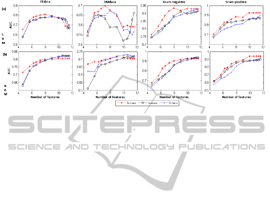
Figure 2: Variation of the performance (AUC values) with the number of features (shown on a log scale) for SVM (a) and

NBM (b) classiﬁers.

that the differences between b-mers and f -mers are

more signiﬁcant than those between b-mers and k-

mers. In other words, b-mers result in better per-

formance as compared to f -mers in more cases than

when we compare them with k-mers. A possible ex-

planation for this is that the ﬁltering criterion that we

use removes some of the informative features (from

b-mers and f -mers sets), while they are present in the

k-mers set. But given that overall the BWT approach

manages to retain more informative features that don’t

overlap much, as opposed to the ﬁltering approach

where more overlapping features are present, for the

same number of features, the b-mers set is generally

better than the f -mers set. However, it is not always

better than the k-mers set, especially for larger fea-

tures sets, as the k-mers set might include informative

features that are not retained in the set of b-mers.

6 CONCLUSIONS AND FUTURE

WORK

6.1 Conclusions

We presented an approach for generating features

for sequence classiﬁcation problems using Burrows

Wheeler Transformation (BWT). This approach can

be seen as a dimensionality reduction technique, as

the features obtained through BWT represent a sub-

set of the set of k-mers, generated using a sliding

window-based approach. To the best of our knowl-

edge, Burrows Wheeler Transformation has never

been used to generate features that are further used

to classify biological sequences. The results of our

experiments on both DNA and protein datasets show

that this attempt of using BWT to generate features

reduces the size of the input feature space, while re-

taining many of the informative features (especially in

the case of protein sequences, where informative fea-

tures are short and appear more frequently throughout

the sequence). Feature selection techniques, applied

on b-mers are faster and give better results as com-

pared to feature selection techniques applied directly

on k-mers. Given all the advantages of the BWT-

based features, we conclude that the BWT approach

can be seen as a powerful tool for generating an initial

pool of features for sequence classiﬁcation problems.

6.2 Future Work

First, given the unsupervised nature of the BWT ap-

proach for generating a reduced set of features, it

would be interesting to investigate the performance

of the features generated using BWT in domain adap-

tation, semi-supervised and transductive settings.

Second, as BWT approach generates mostly non-

overlapping features and could miss informative fea-

ture variations, we would like to investigate the use

of a variant of the BWT approach, where we include

features with mismatches. By allowing certain mis-

matches, we expect an increase in the performance of

the classiﬁers (learned using BWT-based features) es-

pecially for DNA sequence classiﬁcation problems.

Furthermore, a comparison of the BWT-based fea-

tures with k-mers that are grouped together into “mo-

tifs” based on overlaps, as well as with other dimen-

sionality reduction techniques would be another inter-

esting direction for future work.

Given that the best results were obtained with the

SVM algorithm, with default parameters, it would be

BIOINFORMATICS2014-InternationalConferenceonBioinformaticsModels,MethodsandAlgorithms

202

interesting to explore different kernels for SVM, and

perform tuning for different sets of parameters, in or-

der to further improve the performance.

Another interesting direction could be to analyze

the performance of features generated using BWT for

big data, with various feature selection techniques, in

addition to the ECCD technique used in this paper.

ACKNOWLEDGEMENTS

We would like to thank Ana Stanescu in the De-

partment of Computing and Information Sciences

at Kansas State University for making the D.

melanogaster data available for this study. We would

also like to acknowledge Dr. Adrian Silvescu for

insightful discussions regarding the BWT transform,

and Dr. Torben Amtoft for useful discussions regard-

ing time and space complexity of the algorithms stud-

ied in this paper.

REFERENCES

Battiti, R. (1994). Using mutual information for select-

ing features in supervised neural net learning. IEEE

Transactions on Neural Networks, 5:537–550.

Becher, V., Deymonnaz, A., and Heiber, P. (2009). Efﬁ-

cient computation of all perfect repeats in genomic

sequences of up to half a gb, with a case study on the

human genome. Bioinformatics, 25(14):1746–1753.

Burrows, M. and Wheeler, D. J. (1994). A block-sorting

lossless data compression algorithm. Technical Re-

port 124, Digital Equipment Corp., Palo Alto, CA.

Caragea, C., Silvescu, A., and Mitra, P. (2011). Protein

sequence classiﬁcation using feature hashing. In Proc.

of IEEE BIBM 2011, pages 538–543.

Chor, B., Horn, D., Levy, Y., Goldman, N., and Massing-

ham, T. (2009). Genomic DNA k-mer spectra: models

and modalities. GENOME BIOLOGY, 10.

Chuzhanova, N. A., Jones, A. J., and Margetts, S. (1998).

Feature selection for genetic sequence classiﬁcation.

Bioinformatics, 14(2):139–143.

Degroeve, S., De Baets, B., Van de Peer, Y., and Rouz ´e, P.

(2002). Feature subset selection for splice site predic-

tion. Bioinformatics, 18(suppl 2):S75–S83.

Ferragina, P. and Manzini, G. (2000). Opportunistic data

structures with applications. In Proc. of the 41st Symp.

on Foundations of Computer Science, pages 390–398.

Gardy, J. L., Laird, M. R., Chen, F., Rey, S., Walsh, C. J.,

Ester, M., and Brinkman, F. S. L. (2005). Psortb

v.2.0: Expanded prediction of bacterial protein sub-

cellular localization and insights gained from compar.

proteome analysis. Bioinformatics, 21(5):617–623.

Grifﬁth, M., Tang, M. J., Grifﬁth, O. L., Morin, R. D.,

Chan, S. Y., Asano, J. K., Zeng, T., Flibotte, S., Ally,

A., Baross, A., Hirst, M., Jones, S. J. M., Morin,

G. B., Tai, I. T., and Marra, M. A. (2008). ALEXA: a

microarray design platform for alternative expression

analysis. Nature Methods, 5(2):118.

Hall, M., Frank, E., Holmes, G., Pfahringer, B., Reutemann,

P., and Witten, I. H. (2009). The weka data min-

ing software: An update. SIGKDD Explor. Newsl.,

11(1):10–18.

Langmead, B., Trapnell, C., Pop, M., and Salzberg, S.

(2009). Ultrafast and memory-efﬁcient alignment of

short DNA sequences to the human genome. Genome

Biology, 10(3):1–10.

Largeron, C., Moulin, C., and G `ery, M. (2011). Entropy

based feature selection for text categorization. In

Proc. of the 2011 ACM Symp. on Applied Computing,

SAC ’11, pages 924–928, New York, NY, USA. ACM.

Li, H. and Durbin, R. (2009). Fast and accurate short read

alignment with Burrows-Wheeler transform. Bioin-

formatics, 25(14):1754–1760.

Li, R., Li, Y., Kristiansen, K., and Wang, J. (2008). Soap:

short oligonucleotide alignment program. Bioinfor-

matics, 24(5):713–714.

Li, R., Yu, C., Li, Y., Lam, T.-W., Yiu, S.-M., Kristiansen,

K., and Wang, J. (2009). Soap2: an improved ul-

trafast tool for short read alignment. Bioinformatics,

25(15):1966–1967.

Melsted, P. and Pritchard, J. (2011). Efﬁcient counting of

k-mers in dna sequences using a bloom ﬁlter. BMC

Bioinformatics, 12(1):1–7.

Ng, H. T., Goh, W. B., and Low, K. L. (1997). Feature se-

lection, perceptron learning, and a usability case study

for text categorization. SIGIR Forum, 31(SI):67–73.

R ¨atsch, G., Sonnenburg, S., and Sch ¨olkopf, B. (2005).

Rase: recognition of alternatively spliced exons in

c.elegans. Bioinformatics, 21(suppl 1):i369–i377.

Saeys, Y., Rouz `e, P., and Van De Peer, Y. (2007). In search

of the small ones: improved prediction of short exons

in vertebrates, plants, fungi and protists. Bioinformat-

ics, 23(4):414–420.

Salzberg, S. L., Delcher, A. L., Kasif, S., and White,

O. (1998). Microbial gene identiﬁcation using in-

terpolated markov models. Nucleic Acids Research,

26(2):544–548.

Shah, M., Lee, H., Rogers, S., and Touchman, J. (2004). An

exhaustive genome assembly algorithm using k-mers

to indirectly perform n-squared comparisons in o(n).

In Proc. of IEEE CSB 2004, pages 740–741.

Wiener, E. D., Pedersen, J. O., and Weigend, A. S. (1995).

A neural network approach to topic spotting. In Proc.

of SDAIR-95, pages 317–332, Las Vegas, US.

Xia, J., Caragea, D., and Brown, S. (2008). Exploring al-

ternative splicing features using support vector ma-

chines. In Proc. of IEEE BIBM 2008, pages 231–238,

Washington, DC, USA. IEEE Computer Society.

Zavaljevski, N., Stevens, F. J., and Reifman, J. (2002). Sup-

port vector machines with selective kernel scaling for

protein classiﬁcation and identiﬁcation of key amino

acid positions. Bioinformatics, 18(5):689–696.

GeneratingFeaturesusingBurrowsWheelerTransformationfor

BiologicalSequenceClassification

203