
Scalability Analysis of mRMR for Microarray Data
Diego Rego-Fern´andez, Ver´onica Bol´on-Canedo and Amparo Alonso-Betanzos
Department of Computer Science, University of A Coru˜na, Campus de Elvi˜na s/n, A Coru˜na 15071, Spain
Keywords:
Feature Selection, Microarray, Machine Learning, Scalability.
Abstract:
Lately, derived from the Big Data problem, researchers in Machine Learning became also interested not only
in accuracy, but also in scalability. Although scalability of learning methods is a trending issue, scalability of
feature selection methods has not received the same amount of attention. In this research, an attempt to study
scalability of both Feature Selection and Machine Learning on microarray datasets will be done. For this sake,
the minimum redundancy maximum relevance (mRMR) filter method has been chosen, since it claims to be
very adequate for this type of datasets. Three synthetic databases which reflect the problematics of microarray
will be evaluated with new measures, based not only in an accurate selection but also in execution time. The
results obtained are presented and discussed.
1 INTRODUCTION
The advent of DNA microarray technology has
brought the possibility of simultaneously measuring
the expressions of thousands of genes. However, due
to the high cost of experiments, sample sizes of gene
expression measurements remain in hundreds, a very
small number compared to tens of thousands of genes
involved (Mundra and Rajapakse, 2010). Theoreti-
cally, having more genes should give more discrimi-
nating power. But actually, this fact can cause several
problems, such as increasing computational complex-
ity and cost, too many redundant or irrelevant genes
and estimation degradation in the classification er-
ror. Having much higher number of attributes than in-
stances causes difficulties for most machine learning
methods, since they cannot generalize adequately and
therefore, they obtain very poor test performances. To
deal with this problem, and according to Occams ra-
zor (Blumer et al., 1987), the need to reduce dimen-
sionality was soon recognized and several works have
used methods of feature (gene) selection (Saeys et al.,
2007).
Feature selection consists of detecting the rele-
vant features and discarding the irrelevant ones to re-
duce the input dimensionality, and most of the time,
to achieve an improvement in performance (Guyon,
2006). Moreover, several studies show that most
genes measured in a DNA microarray experiment are
not relevant for an accurate distinction among differ-
ent classes of the problem (Golub et al., 1999). To
avoid this curse of dimensionality (Jain and Zongker,
1997), feature selection plays a crucial role in DNA
microarray analysis. Although the efficiency of fea-
ture selection in this domain (and in other areas with
high dimensional datasets), is out of doubt, it is of-
ten forgotten in discussions of scaling, which is an
important issue when dealing with high dimensional
datasets, as it is the case in this research.
Among the different feature selection methods
(Guyon, 2006), filters only rely on general character-
istics of the data, and not on the learning machines;
therefore, they are faster, and more suitable for large
data sets. A common practice in this approach is to
simply select the top-ranked genes where the ranks
are determined by some dependence criteria, and the
number of genes to retain is usually set by human
intuition with trial-and-error. A deficiency of this
ranking approach is that the selected features could
be dependent among themselves. Therefore, a mini-
mum Redundancy Maximum Relevance (mRMR) ap-
proach is preferred in practice (Peng et al., 2005), that
also minimizes the dependence among selected fea-
tures. This filter method has been widely used to deal
with microarray data (Mundra and Rajapakse, 2010;
Zhang et al., 2008; El Akadi et al., 2011). However,
it is a computationally expensive method and its scal-
ability should be evaluated. Therefore, this prelim-
inary research will be focused on the scalability of
the mRMR method over an artificial controlled ex-
perimental scenario, paving the way to its application
to real microarray datasets.
The rest of the paper is organized as follows: sec-
tion 2 describes the mRMR feature selection method,
380
Rego-Fernández D., Bolón-Canedo V. and Alonso-Betanzos A..
Scalability Analysis of mRMR for Microarray Data.
DOI: 10.5220/0004807703800386
In Proceedings of the 6th International Conference on Agents and Artificial Intelligence (ICAART-2014), pages 380-386
ISBN: 978-989-758-015-4
Copyright
c
2014 SCITEPRESS (Science and Technology Publications, Lda.)

section 3 introduces the experimental settings, sec-
tion 4 presents the experimental results and, finally,
section 5 reveals the conclusions and future lines of
research.
2 THE FILTER: mRMR
As mentioned in the Introduction, filters are more
suitable for large datasets, as it is the case in this re-
search. Within filters, one can distinguish between
univariate and multivariate methods (Bol´on-Canedo
et al., 2013). Univariate methods (such as filters
which just evaluate the information gain between a
feature and the class label) are fast and scalable, but
ignore feature dependencies so the features could be
correlated among themselves. On the other hand,
multivariate filters (such as mRMR) model feature de-
pendencies and detect redundancy, but at the cost of
being slower and less scalable than univariate tech-
niques.
To rank the importance of the features of the
datasets included in this research, the mRMR method,
that was first developed by Peng, Long and Ding
(Peng et al., 2005) was used for the analysis of mi-
croarray data. The mRMR method can rank features
based on their relevance to the target, and at the same
time, the redundancy of features is also considered.
Features that have the best trade-off between max-
imum relevance to target and minimum redundancy
are considered as “good” features. The feature selec-
tion purpose is to find maximum dependency, a fea-
ture set S with m features {x
i
}, which have the largest
dependency on the target class c, described by the au-
thors (Peng et al., 2005) as:
max D(S, c), D = I({x
i
, i = 1, ..., m};c)
Implementing the maximum dependency criterion
is not an easy-to-solve task because of the charac-
teristics of high-dimensional spaces. Specifically,
the number of samples is often insufficient and,
moreover, estimating the multivariate density usually
implies expensive computations. An alternative is
to determine the maximum relevance criterion. The
maximum relevance consists of searching features
which satisfy the following equation:
maxD(S, c), D =
1
|S|
∑
x
i
∈S
I(x
i
;c) (1)
Selecting the features according to the maximum
relevance criterion can bring a large amount of
redundancy. Therefore, the following criterion of
minimum redundancy must be added, as suggested
by (Peng et al., 2005) :
min R(S), R =
1
|S|
2
∑
x
i
,x
j
∈S
I(x
i
, x
j
)
Combining the above two criteria and trying to
optimize D and R at the same time, the criterion
called minimum redundancy maximum relevance
(mRMR) arises.
max Φ(D, R), Φ = D− R
In practice, the next incremental algorithm can be
employed:
max
x
j
∈X−S
m−1
[I(x
j
;c) −
1
m−1
∑
x
i
∈S
m−1
I(x
j
;x
i
)]
As mentioned above, mRMR is a multivariate
method so it is expected to be slow and its scalabil-
ity might be compromised. For these reason it is very
interesting to perform a scalability study, which will
be presented in next sections.
3 EXPERIMENTAL SECTION
3.1 Materials
Three synthetic datasets were chosen to evaluate the
scalability of mRMR. Several authors choose to use
artificial data since the desired output is known,there-
fore a feature selection algorithm can be evaluated
with independence of the classifier used. Although
the final goal of a feature selection method is to test its
effectiveness over a real dataset, the first step should
be on synthetic data. The reason for this is twofold
(Belanche and Gonz´alez, 2011):
1. Controlled experiments can be developed by sys-
tematically varying chosen experimental condi-
tions, like adding more irrelevant features. This
fact facilitates to draw more useful conclusions
and to test the strengths and weaknesses of the ex-
isting algorithms.
2. The main advantage of artificial scenarios is the
knowledge of the set of optimal features that must
be selected; thus, the degree of closeness to any
of these solutions can be assessed in a confident
way.
The three synthetic datasets selected (SD1, SD2
and SD3) (Zhu et al., 2010) reflect the problematic of
microarray data. They are challenging problems be-
cause of their high number of features (around 4,000)
and the small number of samples (75), besides of a
ScalabilityAnalysisofmRMRforMicroarrayData
381

high number of irrelevant attributes. In this context,
Zhu et al. (Zhu et al., 2010) introduced two new defi-
nitions of multiclass relevancy features: full class rel-
evant (FCR) and partial class relevant (PCR) features.
On the one hand, FCR features are useful for distin-
guishing any type of cancer. On the other hand, PCR
features only help to identify subsets of cancer types.
SD1, SD2 and SD3 are three-class synthetic
datasets with 75 samples (each class containing 25
samples) and 4000 irrelevant features, generated fol-
lowing the directions given in (D´ıaz-Uriarte and
De Andres, 2006). The number of relevant features
is 20, 40 and 60, respectively, which are divided in
groups of 10. Within each group of 10 features, only
one of them must be selected, since they are redun-
dant with each other.
To sum up, the characteristics of these three
datasets are depicted in Table 1, where one can see
the number of features, the number of features and
samples and the relevant attributes which should be
selected by the feature selection method, as well as
the number of full class relevant (FCR) and partial
class relevant (PCR) features. Notice that G
i
means
that the feature selection method must select only one
feature within the i-th group of features.
Table 1: Characteristics of SD1, SD2 and SD3 datasets.
Dataset
No. of No. of Relevant No. of No. of
features samples features FCR PCR
SD1 4020 75 G
1
, G
2
20 –
SD2
4040 75 G
1
− G
4
30 10
SD3
4060 75 G
1
− G
6
– 60
It has to be noted that the easiest dataset in order to
detect relevant features is SD1, since it contains only
FCR features and the hardest one is SD3, due to the
fact that it contains only PCR genes, which are more
difficult to detect.
For assessing the scalability of the mRMR
method, different configurations of these datasets
were used. In particular, the number of features
ranges from 2
6
to 2
12
whilst the number of samples
ranges from 3
2
to 3
5
(all pairwise combinations). No-
tice that the number of relevant features is fixed (2 for
SD1, 4 for SD2 and 6 for SD3) and it is the number
of irrelevant features the one that varies. When the
number of samples increases, the new instances are
randomly generated.
3.2 Evaluation Metrics
At this point, it is necessary to remind that mRMR
does not return a subset of selected features, but a
ranking of the features where the most relevant one
should be ranked first. The goal of this research
is to assess the scalability of mRMR feature selec-
tion method. For this purpose, some evaluation mea-
sures need to be defined, motivated by the measures
proposed in (Zhang et al., 2009). One
error, cover-
age, ranking loss, average precision and training time
were considered. In all measures, feat
sel is the
ranking of features returned by the mRMR method,
feat
rel is the subset of relevant features and feat irr
stands for the subset of irrelevant features. Notice that
all measures mentioned below except training time
are bounded between 0 and 1.
• The one
error measure evaluates if the top-ranked
(the first selected in the ranking) feature is not in
the set of relevant features.
one
error =
1; feat
sel(1) 6∈ ( feat rel)
0;otherwise
• The coverage evaluates how many steps are
needed, on average, to move down the ranking in
order to cover all the relevant features. At worst,
last ranking feature would be relevant so cover-
age would be 1 (since this measure is bounded
between 0 and 1).
coverage =
max( feat
sel( feat rel(i)))
#feat sel
• The ranking loss evaluates the number of irrele-
vant features that are better ranked than the rel-
evant ones. The fewer irrelevant features are on
the top of the ranking, the best classified are the
relevant ones.
ranking loss =
(coverage ∗ #feat
sel) − #feat rel
#feat rel ∗ # feat irr
• The average precision: evaluates the mean of av-
erage fraction of relevant features ranked above a
particular feature of the ranking.
average
precision =
1
#feat rel
∗
∑
j; feat sel( j) ∈ feat rel ∩ j<i
i;f eat rel(i)
• The training time is reported in seconds.
For example, suppose we have 4 relevant fea-
tures, x
1
, . . . , x
4
, 4 irrelevant features, x
5
, . . . , x
8
and the following ranking returned by mRMR:
x
5
, x
3
, x
8
, x
1
, x
4
, x
2
, x
7
, x
6
. In this case, the one
error
is 1, because the first feature in the ranking is not a
relevant one. For calculating the coverage, it is nec-
essary to move down 6 steps in the ranking to cover
all the relevant features. Regarding the ranking
loss,
there are 2 irrelevant features better ranked than the
relevant ones. As for the average
precision, the num-
ber of relevant features ranked above each feature of
the ranking are the following: 0, 0, 1, 1, 2, 3, 4, 4.
ICAART2014-InternationalConferenceonAgentsandArtificialIntelligence
382

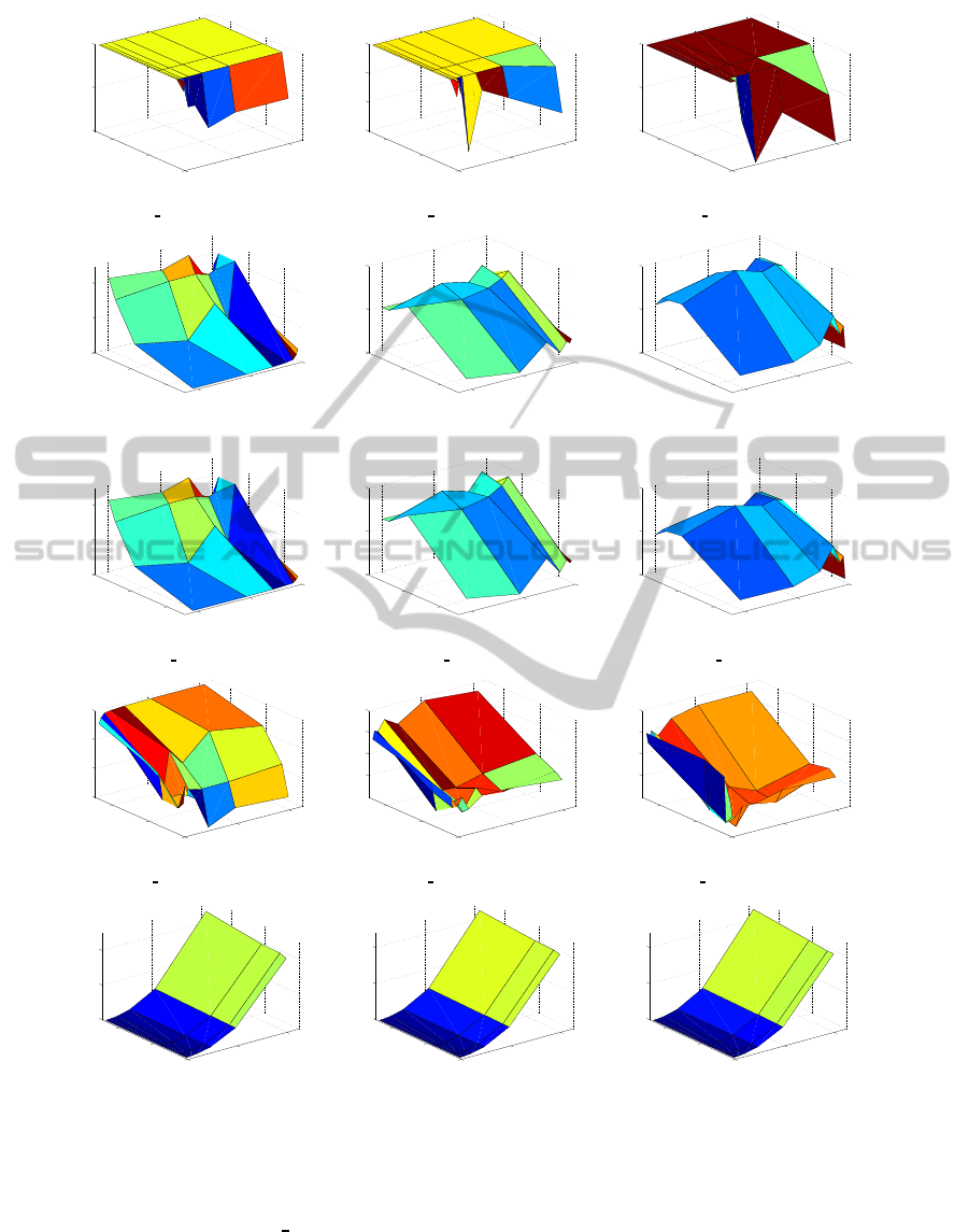
Motivated by the methodology proposed in (Son-
nenburg et al., 2008), we define 5 figures from
which 13 scalar measures are extracted. Note that
the evaluation of mRMR algorithm relies on the bi-
dimensional features-samples space (X-Y -axes). So,
these evaluation measures shape a surface (Z-axis) in
a three-dimensional space.
• One
error surface: Feature size vs Sample size vs
One
error. It is obtained by displaying the evolu-
tion of the One error measure across the feature-
sample space. The following scalar measures are
computed:
1. OeMin: the minimum amount of data (features
x samples) for which the One
error measure
achieves its minimum value.
2. VuOe: volume under the One
error surface.
• Coverage surface: Feature size vs Sample size vs
Coverage. It is obtained by displaying the evo-
lution of the Coverage across the feature-sample
space.
3. Coverage: minimum coverage.
4. Co5%: the minimum amount of data (features
x samples) for which the coverage drops below
a threshold (5% of coverage).
5. VuCo: volume under the coverage surface.
• Ranking
loss surface: Feature size vs Sample size
vs Ranking loss. It is obtained by displaying the
evolution of the ranking
loss across the feature-
sample space.
6. Ranking loss: minimum ranking loss.
7. Rl5%: the minimum amount of data (features x
samples) for which the ranking
loss drops be-
low a threshold (5% of ranking
loss).
8. VuRl: volume under the ranking loss surface.
• Average precision surface: Feature size vs Sam-
ple size vs Average
precision. It is obtained by
displaying the evolution of the average precision
across the feature-sample space.
9. Average precision: maximum aver-
age
precision.
10. Ap95%: the minimum amount of data
(features x samples) for which the aver-
age
precision rises above a threshold (95% of
average
precision).
11. VuAp: volume under the Average
precision sur-
face.
• Training time surface: Feature size vs Sample
size vs Traning time. It is obtained by display-
ing the evolution of the average
precision across
the feature-sample space.
12. Training time: training time in seconds for the
maximum amount of data tested.
13. VuTt: volume under the training time surface.
Those measures related to One
error, Coverage,
Ranking
loss and Training time (i.e. VuOe, Cover-
age, VuCo, Ranking loss, VuRl, Training time and
VuTt) are desirable to be minimized, whilst those re-
lated to Average
precison and amount of data (i.e.
Average precison, VuAp, Co5%, Rl5% and Ap95%)
are desirable to be maximized.
4 RESULTS
This section shows the scalability results for mRMR
according to the measures explained above. Figure 1
plots these measures of scalability after applying a 10-
fold cross validation. Remind that all the metrics but
Average
precision are desirable to be minimized. In
general terms, One error, Coverage and Ranking loss
are more influenced by sample size whilst the training
time is more affected by feature size. In the case of
Average
precision, which should be maximized, this
measure seems to be affected by feature size, since
having more features would make harder the task of
ranking the relevant features on top. Notice that in
the figures related with Coverage and Ranking
loss
the X-Y axes are shifted for visualization purposes.
As expected, the best results on the measures that
assess the adequacy for selecting the most relevant
features in the highest positions of the ranking (Cov-
erage, Ranking
loss and Average precision) are ob-
tained on SD1 (the easiest dataset) whilst the perfor-
mance deteriorates on SD2 and SD3. It has to be no-
ticed that the coverage depends on the dataset, since
the number of relevant features has influence on the
calculation of this measure. Regarding One
error, it
can be seen for all the three datasets that, in most of
the cases, the top ranked feature is not in the subset
of relevant features, which gives an idea of the hard
challenge of the microarray problem.
Regarding the training time (see Figures 1(m),
1(n) and 1(o)), mRMR is sharply affected by the fea-
ture size (as expected for a multivariate filter tech-
nique), remaining almost constant with respect to the
sample size.
Table 2 depicts the thirteen scalar measures related
with Figure 1. These results confirm the trends seen
in Figure 1, reflecting the adequacy of these mea-
sures which are reliable and confident and can give
us a global picture of the scalability properties of the
mRMR filter method. In terms of Coverage and Rank-
ing loss, it can be seen that mRMR achieves good
results, especially on SD1 dataset. In fact, for this
ScalabilityAnalysisofmRMRforMicroarrayData
383
0
2000
4000
0
100
200
0
0.5
1
feat size
sample size
one_error
(a) One error surface in SD1
0
2000
4000
0
100
200
0.4
0.6
0.8
1
feat size
sample size
one_error
(b) One error surface in SD2
0
2000
4000
0
100
200
0.8
0.9
1
feat size
sample size
one_error
(c) One error surface in SD3
0
2000
4000
0
100
200
0
0.2
0.4
feat size
sample size
coverage
(d) Coverage surface in SD1
0
2000
4000
0
100
200
0
0.5
1
feat size
sample size
coverage
(e) Coverage surface in SD2
0
2000
4000
0
100
200
0
0.5
1
feat size
sample size
coverage
(f) Coverage surface in SD3
0
2000
4000
0
100
200
0
0.1
0.2
feat size
sample size
ranking_loss
(g) Ranking loss surface in SD1
0
2000
4000
0
100
200
0
0.1
0.2
feat size
sample size
ranking_loss
(h) Ranking loss surface in SD2
0
2000
4000
0
100
200
0
0.1
0.2
feat size
sample size
ranking_loss
(i) Ranking loss surface in SD3
0
2000
4000
0
100
200
0.7
0.8
0.9
1
feat_size
sample_size
average_precision
(j) Average precision surface in SD1
0
2000
4000
0
100
200
0.7
0.8
0.9
1
feat_size
sample_size
average_precision
(k) Average precision surface in SD2
0
2000
4000
0
100
200
0.7
0.8
0.9
1
feat_size
sample_size
average_precision
(l) Average precision surface in SD3
0
2000
4000
0
100
200
0
500
1000
feat size
sample size
time(s)
(m) Training time surface in SD1
0
2000
4000
0
100
200
0
500
1000
feat size
sample size
time(s)
(n) Training time surface in SD2
0
2000
4000
0
100
200
0
500
1000
feat size
sample size
time(s)
(o) Training time surface in SD3
Figure 1: Measures of scalability of mRMR filter in the SD1 (Figures a, d, g, j and m), SD2 (Figures b, e, h, k and n) and SD3
datasets (Figures c, f, i, l and o).
dataset, the minimum value of these metrics is really
close to zero. As for the Average
precision, it is re-
markable the result obtained on SD1, which obtains a
maximum value very close to one, and an acceptable
value (95 % of the maximum) is achieved with a small
number of data (15552).
Table 3 shows an overview of the behavior of
mRMR according to the different evaluation metrics
over the different datasets studied, where the larger
the number of dots, the better the behavior. To eval-
uate the goodness of the method it was computed a
trade-off between the scalability in terms of number
ICAART2014-InternationalConferenceonAgentsandArtificialIntelligence
384
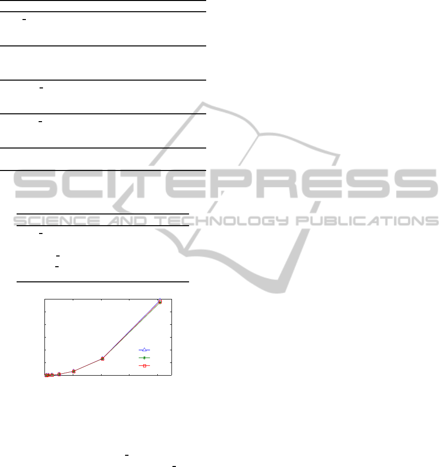
Table 2: Evaluation metrics of mRMR filter in the SD1,
SD2 and SD3 datasets.
Measure SD1 SD2 SD3
One error 0.4 0.5 0.8
Oe5% 9216 4608 9216
VuOe 17.00 17.38 17.70
Coverage 0.0017 0.0293 0.1474
Co5% 995328 497664 497664
VuCo 4.49 9.70 11.79
Ranking loss 0.0006 0.0068 0.0115
Rl5% 995328 497664 15552
VuRl 2.19 2.39 1.93
Average precision 0.9990 0.9893 0.9676
Av95% 15552 124416 248832
VuAp 15.61 13.85 13.25
Training time 1179 1144 1162
VuTt 2577 2577 2589
Table 3: Overview of the behavior regarding scalability of
mRMR on the SD1, SD2 and SD3 datasets.
Measure SD1 SD2 SD3
One error • • •
Coverage ••• •• ••
Ranking
loss •••• ••• •
Average precision •••• ••• ••
Training time ••• ••• •••
0 1000 2000 3000 4000
0
200
400
600
800
1000
1200
feat size
sample size
SD1
SD2
SD3
Figure 2: Training time vs. number of features for mRMR
on SD1, SD2 and SD3 datasets.
of samples and number of features. In this manner, it
is easy to see at a glance that mRMR does not achieve
good results in terms of One
error, whilst shows
strength in terms of Coverage and Ranking loss, es-
pecially with SD1. With regard to the training time,
the difficulty of the dataset has little impact on the
time required to apply the filter, since it is almost con-
stant for the three datasets tested. As can be seen in
Figure 2, the training time is not linear for the num-
ber of features employed. In fact, when using 2000
features, the training time takes around 300 seconds,
while when using double of features (4000), the train-
ing time increases by a factor of four.
5 CONCLUSIONS
With the advent of high dimensional scenarios in ma-
chine learning, scalability is becoming a very impor-
tant trending issue. An algorithm is said to be scalable
if it is suitable, efficient and practical when applied to
large datasets. However, the current state is that the
issue of scalability is far from being solved although
is present in a diverse set of problems such as learn-
ing, clustering or feature selection.
In this research, our attention was focused on the
scalability of feature selection, that has not received
yet as much consideration in the literature as in the
case of learning. In particular, this work is devoted
to analyze the scalability of the well-known mRMR
filter method, which is said to be suitable for microar-
ray datasets. The method was evaluated over three
synthetic datasets which reflect the problematic of mi-
croarray data. For analyzing scalability, these mea-
sures needed to be based not only in the accuracy of
the selection, but also taking into account the execu-
tion time. Finally, the adequacy of the proposed mea-
sures to give a global picture on the mRMR method
on the issue of scalability was shown.
In terms of accuracy of the selection, the mRMR
method was demonstrated to be suitable and scalable
for microarray datasets, since for most of the eval-
uation measures an increase in the amount of data
does not produce a significantly degradation in per-
formance. As for the training time, this filter is multi-
variate, and so the time raises exponentially when the
number of features increases.
For future work, we plan to extend this research
to other datasets and feature selection methods (fil-
ters, wrappers and embedded) in order to draw reli-
able conclusions. A methodology for fusing the pro-
posed evaluation measures seems to be also necessary
when comparing different methods so as to be able to
obtain a ranking of the results, to establish final con-
clusions.
ACKNOWLEDGEMENTS
This research has been partially funded by the Sec-
retar´ıa de Estado de Investigaci´on of the Spanish
Government and FEDER funds of the European
Union through the research project TIN 2012-37954.
Ver´onica Bol´on-Canedo acknowledges the support of
Xunta de Galicia under Plan I2C Grant Program.
ScalabilityAnalysisofmRMRforMicroarrayData
385

REFERENCES
Belanche, L. and Gonz´alez, F. (2011). Review and evalua-
tion of feature selection algorithms in synthetic prob-
lems. arXiv preprint arXiv:1101.2320.
Blumer, A., Ehrenfeucht, A., Haussler, D., and Warmuth,
M. K. (1987). Occam’s razor. Information processing
letters, 24(6):377–380.
Bol´on-Canedo, V., S´anchez-Maro˜no, N., and Alonso-
Betanzos, A. (2013). A review of feature selection
methods on synthetic data. Knowledge and informa-
tion systems, 34(3):483–519.
D´ıaz-Uriarte, R. and De Andres, S. A. (2006). Gene selec-
tion and classification of microarray data using ran-
dom forest. BMC bioinformatics, 7(1):3.
El Akadi, A., Amine, A., El Ouardighi, A., and Abouta-
jdine, D. (2011). A two-stage gene selection scheme
utilizing mRMR filter and ga wrapper. Knowledge and
Information Systems, 26(3):487–500.
Golub, T. R., Slonim, D. K., Tamayo, P., Huard, C., Gaasen-
beek, M., Mesirov, J. P., Coller, H., Loh, M. L., Down-
ing, J. R., Caligiuri, M. A., et al. (1999). Molecu-
lar classification of cancer: class discovery and class
prediction by gene expression monitoring. Science,
286(5439):531–537.
Guyon, I. (2006). Feature extraction: foundations and ap-
plications, volume 207. Springer.
Jain, A. and Zongker, D. (1997). Feature selection: Evalua-
tion, application, and small sample performance. Pat-
tern Analysis and Machine Intelligence, IEEE Trans-
actions on, 19(2):153–158.
Mundra, P. A. and Rajapakse, J. C. (2010). Svm-rfe with
mrmr filter for gene selection. NanoBioscience, IEEE
Transactions on, 9(1):31–37.
Peng, H., Long, F., and Ding, C. (2005). Feature se-
lection based on mutual information criteria of max-
dependency, max-relevance, and min-redundancy.
Pattern Analysis and Machine Intelligence, IEEE
Transactions on, 27(8):1226–1238.
Saeys, Y., Inza, I., and Larra˜naga, P. (2007). A review of
feature selection techniques in bioinformatics. Bioin-
formatics, 23(19):2507–2517.
Sonnenburg, S., Franc, V., Yom-Tov, E., and Sebag, M.
(2008). Pascal large scale learning challenge. In
25th International Conference on Machine Learning
(ICML2008) Workshop. J. Mach. Learn. Res, vol-
ume 10, pages 1937–1953.
Zhang, M.-L., Pe˜na, J. M., and Robles, V. (2009). Feature
selection for multi-label naive bayes classification. In-
formation Sciences, 179(19):3218–3229.
Zhang, Y., Ding, C., and Li, T. (2008). Gene selection al-
gorithm by combining ReliefF and mRMR. BMC ge-
nomics, 9(Suppl 2):S27.
Zhu, Z., Ong, Y.-S., and Zurada, J. M. (2010). Identification
of full and partial class relevant genes. Computational
Biology and Bioinformatics, IEEE/ACM Transactions
on, 7(2):263–277.
ICAART2014-InternationalConferenceonAgentsandArtificialIntelligence
386
