
A Novel Feature Generation Method for Sequence Classification
Mutated Subsequence Generation
Hao Wan, Carolina Ruiz and Joseph Beck
Department of Computer Science, Worcester Polytechnic Institute, Worcester, MA, U.S.A.
Keywords: Sequence Classification, Feature Generation, Mutated Subsequences.
Abstract: In this paper, we present a new feature generation algorithm for sequence data sets called Mutated
Subsequence Generation (MSG). Given a data set of sequences, the MSG algorithm generates features from
these sequences by incorporating mutative positions in subsequences. We compare this algorithm with other
sequence-based feature generation algorithms, including position-based, -grams, and -gapped pairs. Our
experiments show that the MSG algorithm outperforms these other algorithms in domains in which
presence, not specific location, of sequential patterns discriminate among classes in a data set.
1 INTRODUCTION
Finding useful patterns in sequential data is an active
research area. Within this area, supervised sequence
classification deals with the problem of learning
models from labelled sequences. The resulting
models can be used to assign appropriate class labels
to unlabelled sequences. Sequence classification
methods can be used for example to predict whether
a segment of DNA is the promoter region of a gene
or not.
In general, sequence classification is more
difficult than classification of tabular data, mainly
because of two reasons: in sequence classification, it
is unclear what features should be used to
characterize a given data set of sequences (Figure 1
shows three different candidate features whose
presence, or lack of, in a sequence can be used to
characterize the sequence); and the number of such
potential features is very large. For instance, given a
set of sequences of maximum length , over an
alphabet , where
|
|
, if subsequences that
contain symbols are considered as features, then
there are
potential features. Furthermore, the
number of potential features will grow exponentially
as the length of subsequences under consideration
increases, up to
. Thus, how to obtain features
from sequences is a crucial problem in sequence
classification.
A mutation is a change in an element of a
sequence. Like in DNA sequences, this could result
from unrepaired damage to DNA or from an error
when it is replicating itself. We are interested in
whether these changes affect the sequences’
function. Thus, our research focuses on generating
features that represent mutation patterns in the
sequences; and on selecting the generated features
that are most suitable for classification.
More specifically, our proposed algorithm
generates features from sequence data by regarding
contiguous subsequences and mutated subsequences
as potential features. Briefly, it first generates all
contiguous subsequences of a fixed length from the
sequences in the data set. Then it checks whether or
not each pair of candidate feature subsequences that
differ in only one position should be joined into a
mutated subsequence. The join is performed if the
resulting joint mutated subsequence has a stronger
association with the target class than the two
subsequences in the candidate pair do. If that is the
case, the algorithm keeps the joint subsequence and
removes the two subsequences in the candidate pair
from consideration. Otherwise, the algorithm keeps
the candidate pair instead of the joint mutated
subsequence. After all the generated candidate pairs
of all lengths have been checked, a new data set is
constructed containing the target class and the
generated features.
The features in the resulting data set represent
(possibly mutated) segments of the original
sequences that have a strong connection with the
sequences’ function. We then build classification
68
Wan H., Ruiz C. and Beck J..
A Novel Feature Generation Method for Sequence Classification - Mutated Subsequence Generation.
DOI: 10.5220/0004808200680079
In Proceedings of the International Conference on Bioinformatics Models, Methods and Algorithms (BIOINFORMATICS-2014), pages 68-79
ISBN: 978-989-758-012-3
Copyright
c
2014 SCITEPRESS (Science and Technology Publications, Lda.)

models over the new data set that are able to predict
the function (i.e., class value) of novel sequences.
The main contributions of this paper are the
introduction of a new feature generation method
based on mutated subsequences for sequence
classification, and a comparison of the performance
of our algorithm with that of other feature generation
algorithms.
The rest of this paper is organized as follows:
section 2 surveys related work; section 3 provides
background on the techniques used in this paper;
section 4 describes the details of our algorithms;
section 5 compares the performance of our algorithm
with that of other sequence-based feature generation
algorithms from the literature; and section 6
provides some conclusions and future work.
2 RELATED WORK
Feature-based classification algorithms transform
sequences into features for use in sequence
classification (Xing, Pei, & Keogh, June 2010). A
number of feature-based classification algorithms
have been proposed in the literature. For example, k-
grams are substrings of k consecutive characters,
where k is fixed beforehand, see Figure 1(a).
Damashek used -grams to calculate the similarity
between text documents during text categorization
(Damashek, 1995). In (Ji, Bailey, & Dong, 2005),
the authors vary k-grams by adding gap constraints
into the features, see Figure 1(b). Another kind of
feature, k-gapped pair, is a pair of characters with
constraint
, where k is a constant, and
and
are the locations in the sequence where the
characters in the pair occur, see Figure 1(c). The k-
gapped pair method is used to generate features for
Support Vector Machines in (Chuzhanova, Jones, &
Margetts, 1998) and (Huang, Liu, Chen, Chao, &
Chen, 2005). In contrast with our method, the
features generated by their approach can not
represent mutations in the sequences.
Another method is mismatch string kernel
(Leslie, Eskin, Cohen, Weston, & Noble, 2004). It
constructs a (k, m) – mismatch tree for each pair of
sequences to extract k-mer features with at most m
mismatches. It then uses these features to compute
the string kernel function. A similarity between this
method and our method is that both generate
features that are subsequences with mutations.
However, there are three major differences between
them.
1) In mismatch string kernel, the features are
generated from pairs of sequences and used to
update the kernel matrix. In contrast, our MSG
method generates features from the entire set of
data sequences in order to transform the
sequence data set into a feature vector data set.
2) In the process of computing candidate mutated
subsequences, our MSG method does not only
consider mutations in the subsequences, but also
takes into account correlations between these
mutated subsequences and the target classes. In
contrast, the mismatch string kernel method
disregards the latter part.
3) The mismatch string kernel method can be used
in support vector machines and other distance
based classifiers for sequence data. Our MSG
approach is more general as it transforms the
sequences into feature vectors. In other words,
the data set that results from the MSG
transformation can be used with any classifier
defined on feature vectors.
Figure 1: Example of different candidate features for a
given sequence. (a) 4-grams: AACT; (b) 4-grams with gap
1: g(TAAG,1); (c) 2-gapped pair: k(TA,2).
3 BACKGROUND
3.1 Feature Selection
Feature selection methods focus on selecting the
most relevant features of a data set. These methods
can help prediction models in three main aspects:
improving the prediction accuracy; reducing the cost
of building the models; and making the models, and
even the data, more understandable.
To obtain the features that maximize
classification performance, every possible feature set
should be considered. However, exhaustively
searching all the feature sets has been known as a
NP-hard problem (Amaldi & Kann, 1998). Thus, a
number of feature selection algorithms has been
developed, based on greedy search methods like
best-first and hill climbing. See (Kohavi & Johnb,
1997). These greedy algorithms use three main
search strategies: forward selection, backward
deletion, and bi-directional selection.
Forward Selection: it starts at a null feature set. In
each step, the importance of each unselected
feature is calculated according to a specified
metric, and then the most important feature is
added into the feature set. This will go on until
ANovelFeatureGenerationMethodforSequenceClassification-MutatedSubsequenceGeneration
69

there is no important feature to be added.
Backward Deletion: it starts at the full feature set,
and in each step, it removes an unimportant feature
from the feature set, until there is no more
unimportant feature in the remaining feature set.
Bi-directional Selection: it also starts at a null
feature set. In each step, it first applies forward
selection on the unselected features, then it uses
backward deletion on the selected features. This
ends when a stable feature set is reached.
3.2 CFS Evaluation
The Correlation-based Feature Selection (CFS)
algorithm introduces a heuristic function for
evaluating the association between a set of features
and the target classes. It selects a set of features that
are highly correlated with the target classes, yet
uncorrelated with each other. This method was
introduced in (Hall & Smith, 1999). In this paper,
we use this algorithm to select a subset of the
generated features that is expected to have high
classification performance.
3.3 GINI Index
In decision tree induction, the GINI Index is used to
measure the degree of impurity of the target class in
the instances grouped by a set of attributes (Gini,
1912). Similarly in our research, the GINI Index is
used to measure the strength of the association
between candidate features and the target class.
Specifically, we use it during feature generation to
determine whether or not to replace a pair of
subsequences (candidate features) that differ just in
one position with their joined mutated subsequence.
Details are described in section 4.1.3. The GINI
Index of a data set is defined as: 1
∑
∈
,
where is the set of all target classes, and denotes
probability (estimated as frequency in the data set).
Given a discrete feature (or attribute) , the data set
can be partitioned into disjoint groups by the
different values of X. The GINI Index can be used
to calculate the impurity of the target class in each of
these groups. Then, the association between and
the target class can be regarded as the weighted
average of the impurity in each of the
groups:
∑
∗
1
∑
|
∈
.
∈
4 OUR MSG ALGORITHM
4.1
Feature Generation
Our Mutated Subsequence Generation (MSG)
algorithm belongs in the category of feature-based
sequence classification according to the
classification methods described in (Xing, Pei, &
Keogh, June 2010). The MSG algorithm transforms
the original sequences into contiguous subsequences
and mutated subsequences, which are used as
candidate features in the construction of
classification models.
The MSG algorithm generates features of
different lengths according to two user-defined
parameters: the minimum length
and the
maximum length
. The MSG algorithm first
generates the candidate subsequences of length
,
then length
1, and all the way to the
subsequences of length
. Then it takes the union
of all the generated subsequences of different
lengths. Finally, the MSG algorithm constructs a
new data set containing a Boolean feature for each
generated subsequence. Each sequence in the
original data set is represented as a vector of 0’s and
1’s in the new data set, where a feature’s entry in
this vector is 1 if the feature’s corresponding
subsequence is present in the sequence, and 0 if not.
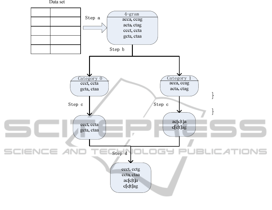
The feature generation process consists of five
main steps described below. Figure 2 shows an
example of the transformation of a sequence data set
into the subsequence features, from Step to Step .
a) The MSG algorithm generates all the
contiguous subsequences of a specific length from
each original sequence (see section 4.1.1);
b) It divides the contiguous subsequences into
categories according to which class they are most
frequent in. is the number of different classes
(see section 4.1.2);
c) For each category, it generates the mutated
subsequences based on the GINI measure (see
section 4.1.3);
d) It combines together all the features from each
category (see section 4.1.4).
e) It repeats Step a to Step d with a different
length, until features of all the lengths in the user
defined range are generated. Then it combines
these features prior to constructing the new data set
(see section 4.1.5).
BIOINFORMATICS2014-InternationalConferenceonBioinformaticsModels,MethodsandAlgorithms
70
Class Sequence
1 accag
1 actag
0 ccctg
0gctaa
ccag
ctag
c[c|t]ag
acca
acta
ac[c|t]a
Figure 2: This figure illustrates the mutated subsequence generation process from Step a) to Step d). In this example,
features of length 4, including mutated subsequences and contiguous subsequences, are obtained. Here, the GINI Index of
each of the mutated subsequences (ac[c|t]a and c[c|t]ag) is better than the GINI Indexes of its forming contiguous
subsequences.
4.1.1 Computation of Contiguous
Subsequences
Contiguous Subsequence: given 1, a contiguous
subsequence of length is a subsequence formed by
taking consecutive symbols from the original
sequence. For example, is a contiguous
subsequence of length 2 in the sequence , while
is not.
Mutated Subsequence: a mutated subsequence is
a subsequence of length (1) which contains
mutative positions, where 1. In each
mutative position, there are two or more
substitutions. In this paper, we consider mutated
subsequences with only one mutative position. For
example, in the subsequence|, the second
position is a mutative position, with two possible
substitutions and . Thus, a mutated subsequence
has many representations, in our example and
. We say that a mutated subsequence is
contained in an original sequence when any of its
representations is contained in the original sequence.
For example, the mutated subsequence | is
contained in the sequence , as well as in the
sequence .
The MSG algorithm starts with the generation of
contiguous subsequences. Suppose that the original
sequences have length , and that the contiguous
subsequences to be computed have length . First,
each sequence is traversed and all of its contiguous
subsequences of symbols are extracted from
starting locations 1 through (1). Then,
duplicate subsequences are removed. For example,
the features in Table 1 are contiguous subsequences
of length 4 for the sequences of the data set in Figure
2. The table also includes the number of occurrences
of each feature in data set sequences of a given
target class.
ANovelFeatureGenerationMethodforSequenceClassification-MutatedSubsequenceGeneration
71

Table 1: contiguous subsequences of length 4 and their
frequency in each class of the data set in Figure 2.
Feature Class 0 Class 1
acca 0 1
ccag 0 1
acta 0 1
ctag 0 1
cact 1 0
actg 1 0
gcta 1 0
ctaa 1 0
4.1.2 Separation
In this step, the algorithm separates the contiguous
subsequences into categories. is the number of
different classes in the data set. Each subsequence is
assigned to a category according to which class it is
most frequent in. For example, the first four features
in Table 1 are assigned to Category 1, because they
are more frequent in Class 1 than in Class 0, and the
other four to Category 2. If a subsequence is
maximally frequent equally in more than one class,
it is randomly assigned to one of those classes.
4.1.3 Generation of Mutated Subsequences
Candidate pair: a candidate pair is a pair of
subsequences which are different from each other in
only one position. For instance, ′′ and ′′ is
a candidate pair. The candidate pair could also
contain mutated subsequences, like for instance
′′ and |.
Joinable checking: joinable checking is used to
determine whether or not to join a candidate pair of
subsequences together, depending on their
correlation with the target class. In this paper, we
use GINI to measure this correlation. For example,
suppose 1 is and 2 is in Table 1.
Their joint sequence 3 is |. By matching
them to the original sequences of the data set in
Figure 2, the data is split into two groups by each
one of these sequences: one group consists of the
original sequences which contain the subsequence,
marked as
; the other group consists of the
rest of sequences, marked as
. Taking
1 as an example, there is only one sequence in
, and it is in class 1; there are three
sequences in
, two of which are in class 0,
and the other one is in class 1. Thus, by using the
formula in section 3.3, we can calculate the GINI
Index for 1 as followings:
1
0
1
1
1
0
1
1
3
2
3
0.444
1
∗
∗
0∗
1
4
0.44∗
3
4
0.333
Similarly, we get the values
2
0.333,
3
0. Since 3 has the best measure
value, implying that it has the strongest association
with the target class, then the candidate pair 1
and 2 is joinable.
In this step, MSG performs joinable checking on
every candidate pair in each category. Once a
candidate pair is determined to be joinable, then the
two subsequences are joined together to create a new
subsequence, called , and they are also marked.
Then the joinable checking is performed on
with every other subsequence in the category. If
there are other subsequences that are joinable with
, then they are also joined together with
and marked. Finally, is added into the mutated
subsequence set. After all candidate pairs are
checked, the algorithm deletes the marked
subsequences and the duplicate mutated
subsequences. The pseudo code of mutated
subsequences generation is shown in Figure 3.
4.1.4 Combination of Categories
In the previous step, some contiguous subsequences
might remain intact. That is, they are not joined with
other subsequences. Thus, in each category, there
might be two types of features: mutated
subsequences and unchanged contiguous
subsequences. In this step, the algorithm combines
the feature sets of all categories together into one
feature set. In this set, all features have length, as
defined in Step 4.1.1.
Table 2: Transformed data set obtained by applying MSG to the data set in Figure 2, with subsequence length 3 and 4.
original
sequence
taa gct ctg cac act cca acc [t|c]ag ctaa gcta actg cact c[t|c]ag ac[t|c]a Class
accag 1 0 0 0 0 0 1 1 1 0 0 0 0 1 1 1
actag 2 0 0 0 0 1 0 0 1 0 0 0 0 1 1 1
ccctg 3 0 0 1 1 1 0 0 0 0 0 1 1 0 0 0
gctaa 4 1 1 0 0 0 0 0 0 1 1 0 0 0 0 0
BIOINFORMATICS2014-InternationalConferenceonBioinformaticsModels,MethodsandAlgorithms
72

Figure 3: The pseudo code for mutated subsequences
generation. ⊕ is the join operator. For example,
⊕
|
and. ⊕
|
|
|
.
4.1.5 Combination of Features of Different
Length
After all the features of the lengths in the user-
defined range are generated in Step 4.1.1 through
Step 4.1.4, the MSG combines these features of
different lengths together and constructs a new data
set with them by matching them to the original
sequence data. In this new data set, each data
instance corresponds to a sequence in the original
data set. The instance’s value for each feature is a
Boolean value describing whether or not the feature
is a subsequence of the instance. Table 2 shows the
transformed data from the data set in Figure
Figure 2
in the range of length 3-4.
4.2 Feature Selection
In this paper, we use bi-directional feature selection
based on the CFS evaluation, as described in section
3, to select the best feature set from the transformed
data set. This feature set is then used to build
classification models.
5 EXPERIMENTAL
EVALUATION
The performance of our MSG algorithm is compared
with that of other feature generation algorithms
which are commonly used for sequence
classification. Such algorithms are:
Position-based (Dong & Pei, 2009): each position
is regarded as a feature, the value of which is the
alphabet symbol in that position.
-grams (Chuzhanova, Jones, & Margetts, 1998):
a -gram is a sequence of length over the
alphabet of the data set. The value of a -gram
induced feature for a sequence S is whether the -
gram occurs in S or not.
-gapped pair (Park & Kanehisa, 2003): in a -
gapped pair,, is an ordered pair of letters
over the alphabet of the data set, is a non-
negative integer. The value of a -gapped pair
induced feature for a sequence is 1 if there is a
position in , where
and
.
Otherwise, the value is 0.
To compare the performance of these algorithms,
a number of experiments are carried out on three
data sets, the first two are collected from UCI
Machine Learning Repository (Bache & Lichman,
2013), and the third one was collected in our prior
work (Wan, Barrett, Ruiz, & Ryder, 2013) from
WormBase (WormBase, 2012):
E.coli promoter gene sequences data set: this
data set consists of 53 DNA promoter sequences
and 53 DNA non-promoter sequences. Each
sequence has length 57. Its alphabet is {a, c, g, t}.
Primate splice-junction gene sequences data set:
this data set contains 3190 DNA sequences of
length 60. Also, its alphabet is {a, c, g, t}. Each
sequence is in one of three classes: exon/intron
boundaries (EI), intron/exon boundaries (IE), and
non-splice (N). 745 data instances are classified as
EI; 751 instances as IE; and 1694 instances as N.
C.elegans gene expression data set: this data set
contains 615 gene promoter sequences of length
1000. We use here expression in EXC cells as the
classification target. 311 of the genes in this data
set are expressed in EXC cells, and the other 304
genes are not.
The performance comparison in the following
sections focuses on the prediction level of models
built on the generated features, and on differences
among the models. We implemented the four feature
generation methods, MSG, k-grams, position-based,
and k-gapped pairs, in our own Java code. To
measure the prediction level, we utilize The WEKA
Procedure: Mutated_Gen(C): generate
the mutated subsequences from
subsequence set C
Initialization: S <- {}
for each pair of subsequences,
sub1 and sub2, in C do
if sub1 and sub2 is joinable
then
sub3 <- sub1 ⊕ sub2
mark sub1;
mark sub2;
for each sequence subi in C do
if sub3 and subi is joinable
then
sub3 <- sub3 ⊕ subi
mark subi
end if
end for
S <- S ∪ {sub3}
end if
end for
for each sequence subj in C do
if subj is marked then
C <- C – subj
end if
end for
ANovelFeatureGenerationMethodforSequenceClassification-MutatedSubsequenceGeneration
73

System of version 3.7.7 (Hall, et al., 2009) to build
three types of prediction models: J48 Decision
Trees, Support Vector Machines (SVMs), and
Logistic Regression (LR). We use n-fold cross
validation to test the models. Then we regard the
models’ accuracy as their prediction level. To
measure the difference between two models, we
perform a paired t-test on their n-fold test results,
and use p-value from the paired t-test to determine
whether or not the difference in model performance
is statistically significant.
Figure 4: Patterns taken from (Towell, Shavlik, &
Noordewier, 1990). Promoter sequences share these
segments at the given locations. In these segments, “x”
represents the occurrence of any nucleotide. The location
is specified as an offset from the Start of Transcription
(SoT). For example, “-37” refers to the location 37 base
pair positions upstream from SoT.
5.1 Results on the E.coli Promoter Gene
Sequences Data Set
5.1.1 Patterns from the Literature
As found in the biological literature (Hawley &
McClure, 1983) (Harley & Reynolds, 1987), and
summarized in (Towell, Shavlik, & Noordewier,
1990), promoter sequences share some common
DNA segments. Figure 4 presents some of these
segments. As can be seen in the figure, these
segments can contain mutated positions. Also the
segments are annotated with specific locations
where the segments occur in the original sequences.
This is an important characteristic distinguishing
these segments from the subsequences generated by
our algorithm. The data set constructed by our MSG
algorithm captures only presence of the
subsequences (not their positions) in the original
sequences.
However, after examining the occurrences of the
aforementioned segments in the Promoter Gene
Sequences data set, we found that for the most part
each segment occurs at most once in each sequence.
Hence computational models created over this data
set that deal only with presence of these patterns are
expected to achieve a prediction accuracy similar to
that of computational models that take location into
consideration. Therefore, since the precise location
of the patterns seems to be irrelevant, we expect our
MSG algorithm to perform well on this data set.
5.1.2 Experimental Results
Each of the four feature generation methods under
consideration (MSG, k-grams, position-based, and k-
gapped pair) was applied to the Promoter Gene
Sequence data set separately, yielding four different
data sets. Parameter values used for the feature
generation methods were the following: for MSG,
the range for the length of transformed subsequences
was 1-5; for -grams, 5; and for -gapped,
10. Then, Correlation-based Feature Selection
(CFS), described in section 3.2, was applied to each
of these data sets to further reduce the number of
features. The resulting number of features in each of
the data sets was: 61 for the MSG transformed data
set, 43 for -grams, 7 for position-based, and 29 for
-gapped pair. 5-fold cross validation was used to
train and test the models constructed on each of
these data sets. Three different model construction
techniques were used: J4.8 decision trees, Logistic
Regression (LR), and SVMs. Figure 5 shows the
prediction accuracy of the obtained models. Table 3
depicts the statistical significance of the
performance difference between the models
constructed over the MSG-transformed data set and
the models constructed
over data sets constructed by
other feature generation methods.
From Figure 5, we can observe that the
prediction levels of the models constructed over
features generated by MSG are superior to those of
models constructed on other features. The t-test
results in Table 3 indicate that this superiority of
MSG is statistically significant at the p < 0.05 level
in the cases highlighted in the table. As expected, the
MSG algorithm generates a highly predictive
collection of features for this data set. This is in part
due to the fact that for this data set, the presence
alone, and not location, of certain subsequences (or
segments) discriminates well between promoter and
non-promoter sequences.
BIOINFORMATICS2014-InternationalConferenceonBioinformaticsModels,MethodsandAlgorithms
74

Figure 5: Accuracy of models built on the features from four different feature generation methods (MSG, k-gram, Position-
based, and k-gapped pair), using three classification algorithms on the Promoter Gene Sequences data.
Table 3: p-values obtained from t-tests comparing the
prediction accuracies of models constructed over MSG-
generated features and models constructed over data sets
generated by the other 3 feature generation methods. T-
tests were performed using 5-fold cross-validation over
the Promoter Gene Sequence data set. Highlighted in the
table are the cases in which the superiority of MSG is
statistically significant at the p < 0.05 level.
Baseline: MSG -grams Position-based -gapped pair
p-value: J48 0.08 0.02 0.03
p-value: LR 0.01 0.06 0.01
p-value: SVM 0.08 0.08 0.01
Table 4: Sample features constructed by the MSG
algorithm over the Promoter Gene Sequences data set,
together with their correlation with the class feature.
MSG features Correlation with target
at[t|a]
-0.37
ccc[a|g]
-0.41
t[t|a]ta
-0.61
[a|c]aaa
-0.58
aaa[g|a|t|c]t
-0.50
ta[a|g|c|t]aa
-0.58
ct[g|t|c|a]tt
-0.41
at[g|a|c]at
-0.51
ata[t|c|a|g]t
-0.53
tta[t|a|c]a
-0.44
aatt[c|a|t|g]
-0.51
a[a|g|c|t]aat
-0.56
aaa[t|c|a|g]c
-0.44
c[a|c|g|t]ggt
0.42
tgag[g|a]
0.43
5.2 Results on the Primate
Splice-Junction Gene Sequences
Data Set
5.2.1 Patterns from the Literature
Some patterns in this data set have been identified in
the literature (Noordewier, Towell, & Shavlik,
1991). Briefly, these patterns state that a sequence is
in EI or IE classes if the triple nucleotides, known as
stop codons, are absent in certain positions of the
sequence. Such triplets are “TAA”, “TAG”, and
“TGA”. Conversely, if a sequence contains any stop
codons in certain specified positions, then the
sequence is not an EI (or IE) sequence. To examine
the effect of position in the patterns, we generated
the following rules, and calculated their confidence
(that is, prediction accuracy) on this data set.
Stop codons are present → not EI (74%)
Stop codons are present at specified positions
→ not
EI (95%)
Stop codons are present → not IE (77%)
Stop codons are present at specified positions → not
IE (91%)
As can be seen, the position information is very
important in these patterns. Hence, we might expect
that the MSG algorithm will not perform well on this
data set, because its generated features do not
contain information about the location where
subsequences appear in the original sequences.
60
70
80
90
100
MSG k‐grams Position‐based k‐gappedpair
Accuracy
Accuracy:J48 Accuracy:LR Accuracy:SVM
ANovelFeatureGenerationMethodforSequenceClassification-MutatedSubsequenceGeneration
75

Figure 6: Accuracy of models built on the features from four different feature generation methods (MSG, k-gram,
Position-based, and k-gapped pair), using three classification algorithms on the Splice-junction Gene Sequence data.
Table 5: p-Values obtained from t-tests comparing the
prediction accuracies of models constructed over MSG-
generated features and models constructed over data sets
generated by the other 3 feature generation methods. T-
tests were performed using 10-fold cross-validation over
the Splice-junction Gene Sequences data set. Highlighted
in the table are the cases in which the superiority of MSG
is statistically significant at the p < 0.05 level.
Baseline: MSG -grams Position-based -gapped pair
p-value: J48 0.23 6.5E-18 2.12E-13
p-value: LR 0.72 6.78E-16 7.3E-13
p-value: SVM 0.15 2.3E-17 3E-14
Table 6: Sample features constructed by the MSG
algorithm over the Splice-junction Gene Sequences data
set, together with their correlation with the class feature.
MSG features Correlation with target
GT[A|G]A
-0.35
GGT[A|G]
-0.38
[G|T|A]GGTA
-0.32
GTA[G|A]G
-0.34
GTG[C|A]G
-0.35
GT[A|G]AG
-0.50
GGT[A|G]A
-0.44
AGGT[A|G]
-0.35
[T|C]AG
-0.02
T[C|T]TC
0.01
TC[T|C]T
-0.03
5.2.2 Experimental Results
Once again, each of the four feature generation
methods under consideration (MSG, k-grams,
position-based, and k-gapped pair) was applied to
the Splice-junction Gene Sequences data set
separately, yielding four different data sets. As in
section 5.1.2, the parameters used for the feature
generation algorithms were: for MSG, the range for
the length of transformed subsequences was 1-5; for
-grams, 5; and for -gapped, 10. Then,
Correlation-based Feature Selection (CFS),
described in section 3.2, was applied to each of these
resulting data sets. The size of the feature set
generated by the MSG algorithm was 28, by -
grams was 29, by position-based was 22, and by -
gapped pair was 49.
10-fold cross validation was used to construct
and test models over these four data sets. Average
accuracies of the resulting models are shown in
Figure 6, and the t-test results in Table 5. On this
data set, the position-based algorithm performed the
best. This is expected given that location
information is relevant for the classification of this
data set’s sequences, as discussed above. The MSG
generated features yielded prediction performance at
the same level of that of k-grams; and statistically
significantly higher performance (at the p < 0.05
significance level) than that of k-gapped pair.
5.3 Results on the C.elegans Gene
Expression Data Set
5.3.1 Patters from the Literature
Motifs are short subsequences in the promoter
sequences that have the ability to bind transcription
factors, and thus to affect gene expression. For
example, a transcription factor CEH-6 is necessary
for the gene aqp-8 to be expressed in the EXC cell,
by binding to a specific subsequence (ATTTGCAT)
in the gene promoter region (Mah, et al., 2010). The
30
40
50
60
70
80
90
100
MSG k‐grams Position‐based k‐gappedpair
Accuracy
Accuracy:J48 Accuracy:LR Accuracy:SVM
BIOINFORMATICS2014-InternationalConferenceonBioinformaticsModels,MethodsandAlgorithms
76

binding sites for a transcription factor are not
completely identical, as some variation is allowed.
These potential binding sites are represented as a
position weight matrix (PWM), see Table 7. A motif
is a reasonable matching subsequence according to a
specific PWM.
It has been shown that motifs at different
locations in the promoter have different importance
in controlling transcription (Reece-Hoyes, et al.,
2007), and that the order of multiple motifs and the
distance between motifs can also affect gene
expression (Wan, Barrett, Ruiz, & Ryder, 2013).
5.3.2 Experimental Results
Once again, each of the four feature generation
methods under consideration (MSG, k-grams,
position-based, and k-gapped pair) was applied to
the C.elegans Gene Expression data set separately,
yielding four different feature vector data sets. The
parameters used for the feature generation
algorithms were: for MSG, the range for the length
of transformed subsequences was 1-6; for -grams,
6; and for -gapped, 10. After CFS, the
size of the feature set generated by the MSG
algorithm was 97, by -grams was 63, by position-
based was 122, and by -gapped pair was 4. The
average accuracies of the resulting models with 10-
fold cross validation are shown in Figure 7.
On this data set, the MSG algorithm produced
the best results, and the p-values in Table 6 indicate
that these results are significantly better than the
results of position-based and k-gapped pair (at the p
< 0.05 significance level). MSG performed slightly
better than k-grams, but not significantly better.
Table 7: A PWM for PHA-4, found in (Ao, Gaudet, Kent,
Muttumu, & Mango, 2004). It records the likelihood of
each nucleotide at each position of the PHA-4 motifs.
A C G T
1 0.097 0.144 0.52 0.238
2 0.003 0.755 0.003 0.238
3 0.003 0.097 0.003 0.896
4 0.003 0.896 0.097 0.003
5 0.003 0.99 0.003 0.003
6 0.849 0.003 0.144 0.003
7 0.99 0.003 0.003 0.003
8 0.614 0.05 0.191 0.144
Table 8: p-Values obtained from t-tests comparing the
prediction accuracies of models constructed over MSG-
generated features and models constructed over data sets
generated by the other 3 feature generation methods. T-
tests were performed using 10-fold cross-validation over
the Gene Expression data set. Highlighted in the table are
the cases in which the superiority of MSG is statistically
significant at the p < 0.05 level.
Baseline: MSG -grams Position-based -gapped pair
p-value: J48 0.18 0.41 0.01
p-value: LR 0.18 6.89E-6 1.45E-5
p-value: SVM 0.21 8.39E-5 4.59E-5
5.4 Discussion
Computational Complexity Comparison of the
Methods. Suppose that a data set consists of
sequences of length , over an alphabet , where
|
|
(for the three data sets considered in this
paper, 4). The position-based method has the
lowest computational complexity out of the four
feature generation methods employed in this
paper. It takes time to extract each location as a
Figure 7: Accuracy of models built on the features from four different feature generation methods (MSG, k-gram, Position-
based, and k-gapped pair), using three classification algorithms on the Gene Expression data.
0,0
10,0
20,0
30,0
40,0
50,0
60,0
70,0
MSG k‐grams Position‐based k‐gappedpair
Accuracy:J48 Accuracy:LR Accuracy:SVM
ANovelFeatureGenerationMethodforSequenceClassification-MutatedSubsequenceGeneration
77

feature for each sequence, so its total complexity is
. K-gapped pair method needs to compute
1 pairs of symbols for each sequence for a
given gap size . In our experiments, we considered
pairs with gap , and since is much less than ,
the time complexity for each sequence is . Its
total complexity is . Similarly, the -gram
method takes time complexity to generate
features of length .
The MSG method has the highest computational
complexity among the four methods. Suppose that
subsequences are given as input to the mutated
subsequences generation process (pseudo code in
Figure 3). There are two outer loops and one inner
loop in this process. The first outer loop goes over
all the
2
pairs of subsequences, and its inner loop
takes at most iterations. The second outer loop
traverses subsequences to delete the marked ones.
So the time complexity of this method is
∗
2
.For a given length , we can
extract at most
subsequences from the sequence
data. Thus, its computational complexity is
in the worst case.
Experimental Comparison of the Methods. The
experimental results on the three data sets above
provide evidence of the usefulness of the proposed
MSG feature generation algorithm. As we discussed
above, patterns in the E.coli promoter gene
sequences data set are position-independent, while
patterns in the primate splice-junction gene
sequences data set are position-dependent. Given
that the MSG-generated features do not take location
into consideration, MSG was expected to perform
very well on the first data set but not on the second
data set. Our experimental results confirm this
hypothesis. In summary, MSG-generated features
are most predictive in domains in which location is
irrelevant or plays a minor role. Nevertheless, even
in domains in which location is important, our MSG
algorithm performed at the same level, or higher,
than other feature generation algorithms from the
literature.
In the C.elegans gene expression data set,
patterns are much more complex than in the other
two data sets considered. Due to the simplicity of the
transformed data set – binary values representing the
presence/absence of features occurring in sequences,
the MSG algorithm does not produce high
classification accuracies on this data set. However,
when compared to the other algorithms under
consideration, MSG generates features that yield
more accurate prediction models. One aspect that
contributes to MSG’s comparably better
performance on this data set is its ability to represent
mutations in the data sequences.
6 CONCLUSIONS AND FUTURE
WORK
In this work, we present a novel feature generation
method, called Mutated Subsequence Generation
(MSG), for feature based sequence classification.
This method considers subsequences, possibly
containing mutated positions, as potential features
for the original sequences. It uses a metric based on
the GINI Index to select the best features. We
compare this method with other feature generation
methods on three genetic data sets, focusing on the
accuracy of the classification models built on the
features generated by these methods. The
experimental results show that MSG outperforms
other feature generation methods in domains where
presence, not specific location, of a pattern within a
sequence is relevant; and can perform at the same
level or higher than other non-position-based feature
generation methods in domains in which specific
location, as well as presence, is important.
Additionally, our MSG method is capable of
identifying one-position mutations in the
subsequence generated features that are highly
associated with the classification target.
Further experimentation on much larger data sets
is needed to confirm the aforementioned findings.
This will be addressed in future work. Other future
work includes a refinement of our MSG algorithm to
reduce its time complexity. We also plan to extend
our MSG method to allow for mutations in more
than one subsequence position. Additionally, we
plan to investigate approaches to and the effects of
incorporating location information in the MSG
generated features.
REFERENCES
Amaldi, E., & Kann, V. (1998). On the approximability of
minimizing nonzero variables or unsatisfied relations
in linear systems. Theoretical Computer Science,
209(1-2), 237–260.
Ao, w., Gaudet, J., Kent, W., Muttumu, S., & Mango, S.
E. (2004, September). Environmentally induced
foregut remodeling by PHA-4/FoxA and DAF-
12/NHR. Science, 305, 1743-1746.
Bache, K., & Lichman, M. (2013). UCI Machine Learning
Repository [http://archive.ics.uci.edu/ml]. Irvine, CA,
BIOINFORMATICS2014-InternationalConferenceonBioinformaticsModels,MethodsandAlgorithms
78

USA: University of California, School of Information
and Computer Science.
Chuzhanova, N. A., Jones, A. J., & Margetts, S. (1998).
Feature selection for genetic sequence classification.
Bioinformatics, 14(2), 139-143.
Damashek, M. (1995, Feb 10). Gauging Similarity with n-
Grams: Language-Independent Categorization of Text.
Science, 267(5199), 843-848.
Dong, G., & Pei, J. (2009). Sequence Data Mining.
Heidelberg: Springer-Verlag Berlin.
Gini, C. (1912). "Italian: Variabilità e
mutabilità"(Variability and Mutability). C. Cuppini,
Bologna, 156 pages. Reprinted in Memorie di
metodologica statistica (Ed. Pizetti E, Salvemini, T).
Rome: Libreria Eredi Virgilio Veschi (1955).
Hall, M. A., & Smith, L. A. (1999). Feature Selection For
Machine Learning: Comparing a Correlation-based
Filter Approach to the Wrapper. Proceedings of the
Twelfth International FLAIRS Conference, (pp. 235–
239). Orlando, FL.
Hall, M., Frank, E., Holmes, G., Pfahringer, B.,
Reutemann, P., & Witten, I. H. (2009). The WEKA
Data Mining Software: An Update. SIGKDD
Explorations, 11(1), 10-18.
Harley, C. B., & Reynolds, R. P. (1987). Analysis of E.
coli promoter sequences. Nucleic Acids Research,
15(5), 2343-2361.
Hawley, D. K., & McClure, W. R. (1983). Compilation
and analysis of Escherichia coli promoter DNA
sequences. Nucleic Acids Research, 11(8), 2237-2255.
Huang, S.-H., Liu, R.-S., Chen, C.-Y., Chao, Y.-T., &
Chen, S.-Y. (2005). Prediction of Outer Membrane
Proteins by Support Vector Machines Using
Combinations of Gapped Amino Acid Pair
Compositions. Proceedings of the 5th IEEE
Symposium on Bioinformatics and Bioengineering
(BIBE’05), (pp. 113-120 ).
Ji, X., Bailey, J., & Dong, G. (2005). Mining Minimal
Distinguishing Subsequence Patterns with Gap
Constraints. Proceedings of the Fifth IEEE
International Conference on Data Mining.
Kohavi, R., & Johnb, G. H. (1997). Wrappers for feature
selection. Artificial Intelligence, 97(1-2), 273-324.
Leslie, C. S., Eskin, E., Cohen, A., Weston, J., & Noble,
W. S. (2004). Mismatch string kernels for
discriminative protein classification. Bioinformatics,
20(4), 467-476.
Mah, A. K., Tu, D. K., Johnsen, R. C., Chu, J. S., Chen,
N., & Baillie, D. L. (2010). Characterization of the
octamer, a cis-regulatory element that modulates
excretory cell gene-expression in Caenorhabditis
elegans. BMC Molecular Biology, 11(19).
Noordewier, M. O., Towell, G. G., & Shavlik, J. W.
(1991). Training Knowledge-Based Neural Networks
to Recognize Genes in DNA Sequences. Advances in
Neural Information Processing Systems, 3.
Park, K.-J., & Kanehisa, M. (2003). Prediction of protein
subcellular locations by support vector machines using
compositions of amino acids and amino acid pairs.
Bioinformatics, 19(13), 1656-1663.
Reece-Hoyes, J. S., Shingles, J., Dupuy, D., Grove, C. A.,
Walhout, A. J., Vidal, M., & Hope, I. A. (2007).
Insight into transcription factor gene duplication from
Caenorhabditis elegans Promoterome-driven
expression patterns. BMC Genomics, 8(27).
Tan, P.-N., Kumar, V., & Steinbach, M. (2005).
Introduction to Data Mining. Boston, MA, USA:
Addison-Wesley.
Towell, G. G., Shavlik, J. W., & Noordewier, M. O.
(1990). Refinement of Approximate Domain Theories
by Knowledge-Based Neural Networks. In
Proceedings of the Eighth National Conference on
Artificial Intelligence, (pp. 861-866).
Wan, H., Barrett, G., Ruiz, C., & Ryder, E. F. (2013).
Mining Association Rules That Incorporate
Transcription Factor Binding Sites and Gene
Expression Patterns in C. elegans. In Proc. Fourth
International Conference on Bioinformatics Models,
Methods and Algorithms BIOINFORMATICS2013
(pp. 81-89). Barcelona, Spain. SciTePress.
WormBase, release WS230. (2012, April 1). Retrieved
from http://www.wormbase.org/
Xing, Z., Pei, J., & Keogh, E. (June 2010). A Brief Survey
on Sequence Classification. ACM SIGKDD
Explorations, 12(1), 40-48.
ANovelFeatureGenerationMethodforSequenceClassification-MutatedSubsequenceGeneration
79
