
Towards Energy-aware Optimisation of Business Processes
Beatriz L
´
opez
1
, Aditya Ghose
2
, Tony Savarimuthu
3
, Mariusz Nowostawski
4
,
Michael Winikoff
3
and Stephen Cranefield
3
1
eXiT research group, University of Girona, Girona, Spain
2
School of Computer Science and Software Engineering, University of Wollongong, Wollongong, Australia
3
Dept. of Information Science, University of Otago, Dunedin, New Zealand
4
Faculty of Computer Science and Media Technology, Gjøvik University College, Gjøvik, Norway
Keywords:
Energy Management, Resource Allocation, Time-dependent Costs, Constraint Optimisation, Auction.
Abstract:
Time dependent energy tariffs are a matter of concern to managers in organisations, who need to rethink how
to allocate resources to business processes so that they take into account energy costs. However, due to the
time-dependent costs, the resource optimisation problem needs to be redesigned. In this paper we formalise
the energy-aware resource allocation problem, including time-dependent variable costs; and present a case
study in which an auction mechanism is used to find a solution. Our results show how the choice of cost
(energy, monetary, or duration) affects the schedules obtained.
1 INTRODUCTION
Increasingly, energy prices are changing from flat
rates to time-dependent tariffs, which presents com-
panies with the problem of smoothing and shifting
peaks from expensive to cheaper hours. Dealing with
time-dependent energy costs has been mainly studied
in the context of household management (Gottwalt
et al., 2011), and business process management has
been mostly neglected. An exception is the proposal
of Hoesch-Klohe et al. (2010) in which resources are
annotated with CO
2
consumption details, which are
known to the process manager that aggregates the en-
ergy costs.
This paper considers allocation and optimisation
of resources in business processes while taking into
account energy costs. Business processes pose partic-
ular challenges to optimisation because, unlike house-
hold energy usage, they are structured (e.g. a process
may involve an extended sequence of steps), and may
include structural uncertainty (e.g. the business pro-
cess may include embedded decisions, so the exact
tasks to be performed will not be known with cer-
tainty ahead of time).
The key contribution of the work is the problem
formalisation, which includes the optimisation of re-
sources taking into account time-dependent energy
costs. With the formalisation of the problem, we aim
to provide a new optimisation problem to the research
arena, the solution of which will provide new tools for
business managers to support energy-aware decision-
making.
We also provide an auction-based resource-
allocation mechanism to illustrate with a case study
the possible outcomes of the energy-aware optimisa-
tion process. However, the focus of the paper is not
the technological part (auction-based resource alloca-
tion), but to provide a first approach to formalising
the problem of energy-aware optimisation of business
processes.
This paper is organised as follows. First we start
by reviewing related work in Section 2. Next, in Sec-
tion 3 we provide the formalisation of the energy-
aware resource optimisation problem. In Section 4
a case study is provided, and we end in Section 5 with
some discussion and ideas for further research.
2 RELATED WORK
Research on green business process management is
described by Nowak et al. (2011) , who identify the
required changes for business processes to be envi-
ronmentally aware. Focusing on energy, Ardagna et
al. (2008) propose a framework that includes a con-
trol layer in which the energy consumption is opti-
mized according to execution times. In subsequent
68
López B., Ghose A., Savarimuthu T., Nowostawski M., Winikoff M. and Cranefield S..
Towards Energy-aware Optimisation of Business Processes.
DOI: 10.5220/0004809700680075
In Proceedings of the 3rd International Conference on Smart Grids and Green IT Systems (SMARTGREENS-2014), pages 68-75
ISBN: 978-989-758-025-3
Copyright
c
2014 SCITEPRESS (Science and Technology Publications, Lda.)

work, Cappiello et al. (2010) describe a tool for val-
idating the desired energy consumption. All of these
approaches are based on web services and a task is as-
signed to at most one service. By contrast, our work
allocates a given task to bundles of services (i.e. re-
sources).
The timeline-based scheduling work of Chien et
al. (2010) is similar to our work in that they have
a collection of business process instances, each of
which has resource requirements. A key difference
between their work and ours lies in the fact that they
are able to drop business process instances. Further-
more, we deal with time-dependent costs of resources,
which they do not.
Time-variable cost functions have been recently
considered by the constraint community (Simonis and
Hadzic, 2010), but the solution proposed can only
be applied in centralised environments and is not ap-
plicable to our business process model. More gen-
erally, traditional research on the job shop problem
and workflow resourcing considers a one-to-one map-
ping of tasks to machines, whereas we allow a task
to require multiple resources. Other differences in-
clude our allowance for uncertainty in the workflow
(through the presence of XOR nodes), and our use of
abstract tasks.
3 PROBLEM FORMULATION
We address energy optimisation issues in the context
of resource allocation for business processes. The
main inputs of our problem are the tasks to be per-
formed and their sequencing dependencies, the re-
sources available, constraints on the time and resource
availability, and the cost function that characterizes
the optimisation target.
3.1 Tasks
Formally we define a set of all the task instances in-
volved in a given workload T = {t
1
. . .t
m
}. Each task
has an associated duration that is not fixed, but de-
pends on the resources used. We then define a busi-
ness process instance B as being a graph B = (V, E)
where the vertices are one of the following: a task t
i
,
one of a set of XOR nodes X = {x
1
, . . . , x
k
}, or either
the distinguished start node s or end node e. Formally
V = T ∪X ∪{s, e}. As usual, E is a set of pairs of ver-
tices (v, v
0
) where v, v
0
∈ V . Each XOR node x
i
has an
associated set of options: option(x
i
) = {B
1
x
i
, . . . , B
k
i
x
i
}
where each of the elements of the set B
j
x
i
is a graph,
as defined above. In other words, we have a top-level
graph B which may have some nodes that are them-
selves place-holders for one of a set of sub-graphs.
We require that the tree of graphs is finite—the leaf
graphs are those with no XOR nodes (X = {}).
The interpretation of XOR nodes is that eventu-
ally at run time each x
i
is replaced by one of its sub-
graphs B
0
∈ option(x
i
). This replacement is repeated
until there are no XOR nodes remaining. Since there
is a choice of B
0
∈ option(x
i
) for each x
i
, this process
is non-deterministic. It results in a “decided” graph
which has X = {}, i.e. no XOR nodes.
This run-time recursive replacement of each XOR
node with one of its alternative subgraphs models the
“don’t know” non-determinism of workflow execu-
tion, where there may be different sub-workflows for
performing a complex job, but the one that will be
used for any workflow instance will be decided at run
time (due to resource availability or other situational
factors that we do not attempt to model).
We use v v
0
to denote that there is a path from v
to v
0
, defined in the usual way
1
, and use v
1
v
2
v
3
as shorthand for v
1
v
2
∧ v
2
v
3
.
We require the graph (V, E) to be well-formed,
which we define to mean that there are no arcs to
the start node (¬∃v.(v, s) ∈ E); there are no arcs from
the end node (¬∃v.(e, v) ∈ E); there are no cycles
(¬∃v ∈ V.v v ); and for any node v ∈ V (apart from
the start and end nodes), there is a path from s to v and
from v to e (∀v ∈ (V \{s, e}) . s v e).
3.2 Resources
Each task requires resources in order to be carried
out. We define a set of known resource types RT =
{r
1
, . . . , r
n
}. We use multisets to represent the set of
available resources, AvailRS, and the resources that
are allocated to each task in a process schedule. A
multiset over RT (a “resource multiset”) is defined by
a characteristic function R : RT → N indicating how
many copies of each element of RT appear in the mul-
tiset
2
. For convenience we will write multisets using
standard set notation
3
, but with the possibility of ele-
1
v v
0
≡ (v, v
0
) ∈ E ∨ (∃v
00
.(v, v
00
) ∈ E ∧ v
00
v
0
)
2
This definition of multisets does not allow for real-
valued quantities of resources to be represented, but this
is not a limitation: we could easily extend the notation to
use real numbers, or assume that the unit of measurement
is sufficiently fine grained that natural numbers are not a
limitation, for instance, measuring coal in units of grams.
3
We use standard definitions of multiset relations and
functions (Syropoulos, 2001): R
1
⊆ R
2
= ∀r ∈ RT.R
1
(r) ≤
R
2
(r). We distinguish between a maximum-based set union
(∪) and an accumulating union (]): R
1
∪R
2
= g where ∀r ∈
RT.g(r) = max(R
1
(r), R
2
(r)) and R
1
] R
2
= g where ∀r ∈
RT.g(r) = R
1
(r) + R
2
(r).
TowardsEnergy-awareOptimisationofBusinessProcesses
69

ments appearing multiple times. We will also use the
abbreviation a
n
to represent n copies of an element,
e.g. {a
2
, b} = {a, a, b}.
Each resource type has associated monetary and
energy costs. As discussed earlier, a key require-
ment is that these costs may vary over time. For-
mally we define the monetary cost cost(τ
1
, τ
2
, r
i
) and
energy cost energy(τ
1
, τ
2
, r
i
) as being functions from
a time interval [τ
1
, τ
2
] (i.e. τ
1
≤ t ≤ τ
2
, where τ
1
< τ
2
,
τ
1
, τ
2
∈ N) and a resource type r
i
∈ RT to a cost (a
real number), representing the total cost of one unit
of resource type r
i
over the given time interval.
We also define time-dependent monetary and
energy set-up costs, setup cost(r,t
1
, τ
1
,t
2
, τ
2
) and
setup energy(r,t
1
, τ
1
,t
2
, τ
2
), representing additional
costs (or cost savings) that apply when a resource of
type r is used for a task t
1
starting at time τ
1
and the
next task for the resource is t
2
starting at τ
2
(not nec-
essarily immediately after the end of t
1
). A resource
type r may also have a minimum set-up time that must
be allowed between its use for a task t
1
starting at
τ
1
and its next task t
2
, denoted setup time(r,t
1
, τ
1
,t
2
).
Unlike the set-up cost and set-up energy cost, we as-
sume that this does not depend on t
2
’s starting time.
Note that, because our representation doesn’t dis-
tinguish between different instances of a given re-
source type, set-up costs and times can only be non-
zero for resource types where there is a single instance
available, i.e. AvailRS(r) = 1. We use RT
1
to denote
those resource types for which exactly one instance is
available.
Finally, we generalise the set-up costs
and times to also apply to XOR nodes:
setup cost(r,t
i
, start
i
, x
j
, start
j
) is defined as the
maximal cost over those tasks in the subgraphs of
the XOR node that are initial for r. Given a set
of subgraphs, a task is initial for r if it is possible
for it to be the first task using r to be executed
in one of the subgraphs, i.e. if we only consider
tasks that use r, it is an initial task. We define
setup cost(r, x
j
, start
j
,t
i
, start
i
) in an analogous way
(in terms of tasks in x
j
that are final for r), and extend
this to define the set-up cost between two XOR nodes
in terms of a maximum over the tasks that are final
for r in the set of options for the first XOR node and
those that are initial for r in the set of options for the
second XOR node.
We link tasks and resources by defining need(t
i
)
which denotes the resources that task t
i
requires. In
order to model “don’t care” nondeterminism, where
there are multiple ways of achieving a task, and we
are happy to have the choice be dictated by the needs
of other processes, we define need(t
i
) as a set of al-
ternative requirements. Furthermore, for each alter-
native resource requirement, we also specify the dura-
tion of the task when those resources are allocated to
it. Formally, need(t
i
) = {(R
1
, d
i
1
). . . (R
k
i
, d
i
k
i
)}, where
each R
i
is a multiset and each d
i
j
is a natural num-
ber denoting the duration of task t
i
if the j
th
resource
multiset is used.
3.3 Schedules
A schedule S for a business process assigns to each
task a starting and ending time (respecting the se-
quencing constraints) and resources (such that the
available resources are not exceeded at any point in
time). Formally, a schedule S is a set of task records:
S ={s
1
, . . . , s
m
} ∪ {s
0
1
, . . . , s
0
k
}
∪ {(start
s
, end
s
, {}, s), (start
e
, end
e
, {}, e)}
(1)
There are two types of task records: s
i
which
correspond to tasks, and s
0
j
which correspond to
XOR nodes. A task record s
i
is a tuple s
i
=
(start
i
, end
i
, RS
i
,t
i
) where start
i
is the start time of
the task’s performance, end
i
is the completion time,
RS
i
is a multiset of resources assigned to the task,
and t
i
is the task. For convenience we include task
records for the start and end nodes. These are treated
as tasks that take no time to perform (so start
s
= end
s
and start
e
= end
e
) and have no resource requirements
(so RS
s
= RS
e
= {}). An XOR node record is a tuple
s
0
j
= (start
j
, end
j
, S
j
, x
j
) where start
j
and end
j
are re-
spectively the start and end times, x
j
is the XOR node
identifier, and S
j
is a set of sub-schedules, i.e. a sched-
ule for each sub-graph in option(x
j
). We require that
start
j
must be the smallest of the starting times of a
schedule in S
j
, and similarly end
j
must be the largest
finishing time of a schedule in S
j
.
Schedules are subject to various constraints re-
lated to tasks, set-up times, and resources. First, the
task records in a schedule must satisfy a number of
constraints: (i) each task t
i
has a single correspond-
ing task record s
i
; (ii) each XOR node x
j
has a single
corresponding XOR node record s
0
j
; (iii) each task t
i
is allocated the resources specified by one of the re-
source multisets in need(t
i
), and takes the correspond-
ing specified length of time to be executed
4
; and (iv)
the task start and end times must satisfy the constraint
that (t
i
,t
j
) ∈ E ⇒ end
i
≤ start
j
.
Second, the above constraints on the schedule
need to be extended to respect set-up times: where
a (singleton) resource of type r is used by t
i
and
then by t
j
, the schedule must satisfy the stronger con-
straint end
i
+ setup time(r, t
i
, start
i
,t
j
) ≤ start
j
. Note
4
Formally, for some (R
j
, d
i
j
) ∈ need(t
i
): R
i
= R
j
, and
end
i
− start
i
= d
i
j
.
SMARTGREENS2014-3rdInternationalConferenceonSmartGridsandGreenITSystems
70

that t
i
and t
j
may not be constrained to occur in se-
quence. We therefore define this additional feasibil-
ity constraint using a singleton resource schedule S
r
which, given schedule S and singleton resource type
r, is a list of the task records for those tasks (both s
i
and s
0
j
) that use resource r, sorted by starting time.
The additional feasibility condition is then: ∀r ∈
RT
1
∀(t
i
,t
j
) ∈ S
r
. end
i
+ setup time(r,t
i
, start
i
,t
j
) ≤
start
j
where (t
i
,t
j
) ∈ S
r
denotes the selection of ad-
jacent elements in the list, i.e. S
r
= h. . . ,t
i
,t
j
, . . .i.
Third, having defined the constraints that ensure
a schedule is feasible with respect to time (including
set-up times), we now define the feasibility of a sched-
ule with respect to the available resources (AvailRS).
We begin by defining functions that accumulate the
resources used by a schedule S at time τ:
res(τ, (start
i
, end
i
, RS
i
,t
i
))
=
RS
i
if start
i
≤ τ ≤ end
i
{} otherwise
res(τ, (start
j
, end
j
, S
j
, x
j
)) =
[
s∈S
j
res(τ, s)
Res(τ, S) =
]
s∈S
res(τ, s)
The first function (res) takes a time τ and a task record
s
i
or s
0
j
and returns the resources required for the task
at time τ, which will, for s
i
, be either RS
i
if the task
is being performed at time τ, or the empty set; and
for x
j
is simply the maximum of the resources re-
quired at time τ over the sub-schedules in S
j
(we need
to use the maximum since we do not know which
option will be selected). The second function (Res)
takes a time τ and an entire schedule, and collects
the resource requirements for a given time τ across
all the tasks. Finally, a schedule S is feasible with re-
spect to the available resources AvailRS if and only if
∀τ start
s
≤ τ ≤ end
e
. Res(τ, S) ⊆ AvailRS.
3.4 Optimisation Costs
Finally, we need to define the cost of a given (fea-
sible) schedule. In fact there are three costs that we
consider: the energy cost, the monetary cost, and the
time. The energy cost of a schedule is defined as fol-
lows
5
:
Cost
e
(S) =
∑
s∈S
Cost
e
(s)
+
∑
r∈RT
1
∑
(t
i
,t
j
)∈S
r
setup energy(r,t
i
, start
i
,t
j
, start
j
)
Cost
e
(s
i
) =
∑
r∈RT
RS
i
(r) × energy(start
i
, end
i
, r
j
)
5
For convenience we overload Cost
e
to operate on both
schedule and task records.
Cost
e
((start
j
, end
j
, S
j
, x
j
)) = max
S∈S
j
Cost
e
(S)
Finally, the time cost is simply the makespan:
Cost
t
(S) = end
e
− start
s
In other words, the cost of a schedule is the sum of
the costs for each of the task entries s
i
and the XOR
entries s
0
j
(first term) and the sum of the set-up costs
(second term). Note that because the set-up cost is de-
fined over both task and XOR nodes, and S
r
includes
both types of nodes, the second term includes the set-
up costs between tasks and XOR nodes. To com-
pute the cost of an individual task record, we com-
pute for each resource type the cost of a single unit of
that resource type across the given time interval, and
multiply by the number of resource type units RS
i
(r)
allocated. For XOR records, we take the maximum
across the options. Similarly, we define the monetary
cost, and finally, the time cost is simply the makespan:
Cost
t
(S) = end
e
− start
s
3.5 Problem Statement
Given a workload represented by graph B, the prob-
lem we are tackling is to find a feasible schedule
S which minimises the three cost functions (Cost
e
,
Cost
e
and Cost
t
). This is a multi-criteria optimisation
problem in which we cannot assign a priori a greater
importance to any given criterion, and so we are look-
ing not for a single “optimal” solution, but for a set of
Pareto points.
4 CASE STUDY
In this section we address the problem by means of an
auction mechanism, with the aim of illustrating the
different solution outcomes that arise when each of
the energy, monetary cost, and makespan (i.e. time
cost) are given precedence.
4.1 Auction Implementation
Auctions have been widely used for task and resource
allocation among different entities with the particular-
ity that the price of the resource allocation is decided
when clearing the market (Chevaleyre et al., 2006).
When auctioneers demand tasks to be performed by
bidders (resource agents), the mechanism is known as
a reverse auction. The protocol followed in such auc-
tions includes the main following steps:
1. The auctioneer sends a request for proposal, in
which the tasks to be performed are specified.
TowardsEnergy-awareOptimisationofBusinessProcesses
71
2. The bidders answer with some offers.
3. The auctioneer decides the set of winner bids.
4. The auctioneer acknowledges the winner bidders.
5. The bidders commit the time to perform the tasks.
6. After the tasks have been performed, bidders send
the auctioneer a “done” message that enacts the
last step.
7. The auctioneer pays for the activity performed by
the resources.
To apply an auction mechanism to our problem
there are several choices to be made when designing
the auction.
First, there is the choice of when the allocation
of resources to tasks is performed. Resources can
be scheduled in advance or following a dynamic
approach, interleaving scheduling and execution of
tasks. The latter approach improves the specifications
of the tasks to be performed, since the uncertainty
about which branch of the XOR node will be followed
is cleared before resources are allocated. Due to the
fact that we operate on business process instances and
during the execution of the business process we may
not have a sufficient amount of time to perform the
scheduling, we are interested in solutions where we
conduct scheduling ahead of time and booking of re-
sources is done in advance. This approach requires
us to consider overlapping resource allocation across
tasks that belong to separate exclusive-or paths of the
business process graph.
Second, we can perform a single auction with all
of the tasks involved in a business process, or we can
proceed with a sequential process, auctioning a task
at a time. The latter case is useful if we can ob-
tain a more precise picture of the requirements and
constraints of a task once the preceding tasks have
been allocated, as in the work of Collins and Gini
(2009). However, the presence of XOR and paral-
lel (AND) branches introduces uncertainty on which
tasks should be allocated first. Thus we follow the
first approach: scheduling all of the tasks in a single
auction.
Third, given the set of tasks to be performed, bid-
ders can provide bids on bundles of tasks so that
the resulting mechanism is a combinatorial auction.
Moreover, bidding on bundles enables the resource
to express that the assignment of two (or more) con-
secutive tasks can improve cost, for example, to re-
duce the transport cost of moving some resource to a
given place where the tasks should be performed (set-
up costs).
Fourth, there is a single winner determination
problem (WDP) to be solved. The solution of the
WDP includes the allocation of both start time and
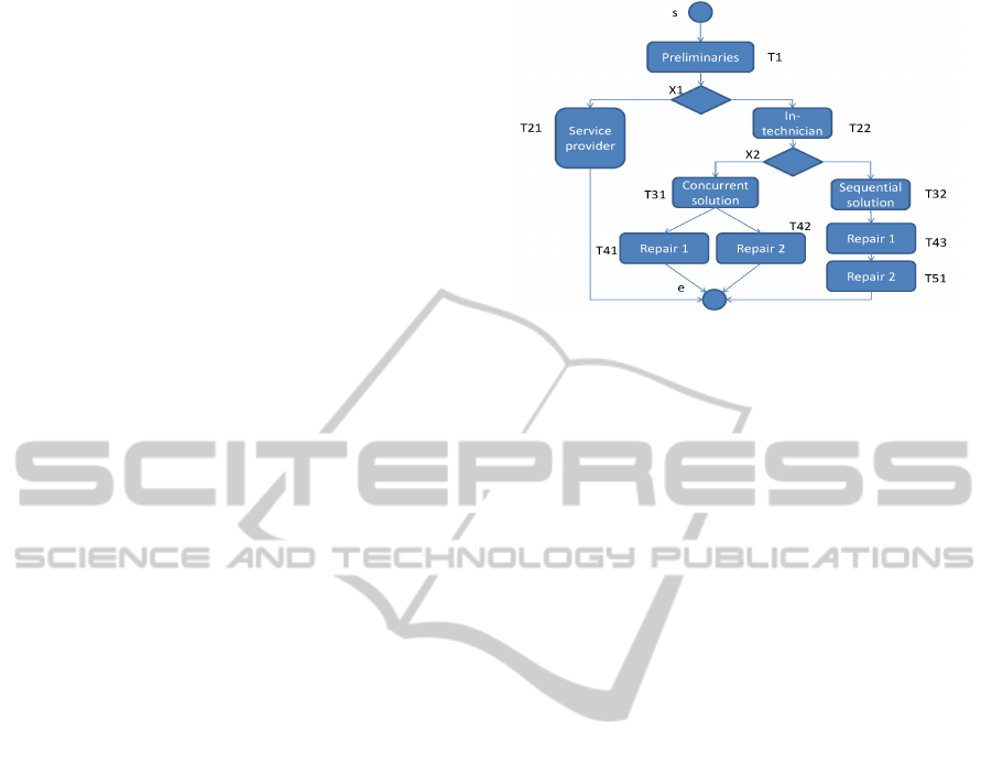
Figure 1: Business process example.
resources, for each of the tasks of a business pro-
cess, taking into account the constraints specified in
the problem formulation. Moreover, and thanks to the
explicit definition of resource bundle alternatives as-
sociated to each task (need(t
i
)), the winner determina-
tion algorithm decides upon a single bundle for a task
based on the bids provided. From this point of view,
the auction model is a combinatorial auction, since the
auctioneer needs to get all of the resources of an al-
ternative (R
j
∈ need(t
i
)), or none of them. Therefore
our auction model is two-fold combinatorial: bidders
bid for bundles of tasks and auctioneers assign tasks
to bundles of resources. This auction model is related
to combinatorial exchanges (Parkes et al., 2001).
Steps four to six of the protocol involve resource
acceptance and deployment after the allocation has
been cleared. We are dealing with a single auction
where no other request, outside this auction, is being
managed by any resource agents. Thus we do not ex-
pect any rejection on behalf of agents. Failures during
the tasks’ execution are out of the scope of this paper
(see the work of Ramchurn et al. (2009) for preventive
issues).
We assume that the final step—the payment
mechanism—is incentive compatible, so all of the re-
source agents provide truthful bids (i.e. they do not
cheat when bidding).
4.2 Results
In this section we provide an auction-based solution
for scheduling resources to the instances of the busi-
ness process given in Figure 1. There are two XOR
nodes X1 and X2. X1 decides whether the branch
containing T21 or the branch containing T22 will be
executed. X2 decides whether the branch containing
T31 or the branch containing T32 will be executed.
Note that tasks T41 and T42 can be executed concur-
rently (i.e. there is an AND split and join).
For each task, the bundles of resources (or single
SMARTGREENS2014-3rdInternationalConferenceonSmartGridsandGreenITSystems
72

Table 1: Resources required by each task.
Task (Resources, Duration)
T1 ({R1}, 1)
T21 ({R2,R1}, 5), ({R2,R3}, 5)
T22 ({R1},1), ({R4},1)
T31 ({R1},1), ({R4},1)
T32 ({R1},1), ({R4},1)
T41 ({R3},2), ({R4},2)
T42 ({R3},3), ({R4},3)
T43 ({R1},2), ({R4},2)
T51 ({R3},1), ({R4},1)
Table 2: Resource costs. Energy is expressed in kWh;
money in euros; duration in hours.
Id kWh e Duration
R1 1 160 (T1,1), (T21,4), (T22,3), (T31,2)
(T32,1), (T43,1)
R2 10 200 (T21,4)
R3 5 90 (T21,4), (T41,3), (T42,4), (T51,1)
R4 3 50 (T22,1), (T31,1), (T32,2), (T41,3),
(T42,3), (T43,4), (T51,2)
resources) that are capable of performing the task and
the expected duration to complete the task (from the
auctioneer’s perspective) are given in Table 1. For
example, task T21 can be performed by two differ-
ent bundles of resources, {R2, R1} or {R2, R3}. The
resource costs (energy costs and monetary costs) are
provided in Table 2. Note that the expected duration
of tasks from an auctioneer’s perspective may or may
not correspond to the actual ability of the resource
agents (i.e. the resource agents may provide a differ-
ent duration as a part of their bids and this information
is internal to a resource agent). For example, the com-
mon information indicates that T21 takes 5 hours re-
gardless of which resource bundle is taken, but the re-
sources themselves indicate that the task actually only
takes 4 hours.
We assume that day-ahead hourly prices (i.e. en-
ergy costs in kW per hour) are available (see Fig-
ure 2). This is similar to the work of Gottwalt et
al. (2011). Additionally, we also assume that the re-
source allocation process starts at 8am.
All the tasks from all of the business process in-
stances are allocated in a single auction. For the busi-
ness process given in Figure 1, there are 9 tasks for
Figure 2: Day-ahead hourly tariffs.
which resources need to be allocated. They are T1,
T21, T22, T31, T32, T41, T42, T43, T51. For each
task, a time window is generated according to the du-
ration estimated by the auctioneer (see Table 1) with
a slack time of 2 hours. For example, since the sched-
ule begins at 8am and T1 takes 1 hour, the request
(T1, [8,11]) is sent to R1.
It should be noted that each agent may receive sev-
eral requests. Agents process the requests and gener-
ate a single bid, which includes the set-up times. We
have considered set-up costs in R4 (between T32 and
T43, and between T43 and T51) and R3 (between T43
and T51). In all of the cases, the set-up cost consists
of an extra monetary, energy and time unit cost.
Once the auctioneer collects all of the bids, the
winner is determined. For determining the winner
of the auction we consider three different scenarios.
These three scenarios consider three attributes: the
energy cost, the monetary cost and the makespan.
However, the relative importance of these attributes
differs in each of the scenarios.
Energy wins: the bid with the cheapest energy cost
is selected. In case of a tie between energy costs, the
one with the cheapest monetary cost will be preferred.
Again if there is a tie, the makespan will be consid-
ered.
Money wins: the bid with the cheapest monetary cost
is selected. In case of ties (the same monetary costs),
energy costs will be considered for comparison. If
there is a tie in energy costs, makespan will be con-
sidered.
Makespan wins: the bid with the shortest makespan
is selected. In case of a tie, the cheapest energy cost is
considered. If there is a tie between energy costs, the
cheapest monetary cost is considered. We consider
the makespan with the starting time that is closest to
the earliest starting time of the activities scheduled for
a given day (i.e. 8am in our case).
We note that six different scenarios can be consid-
ered for a combination of three attributes. In this pa-
per we compare three scenarios, and we believe these
scenarios are sufficient to show the consequences of
using energy costs in resource allocation in business
processes.
The resultant resource allocations at the end of the
auction process for each of the scenarios are shown in
Figure 3. Note that a resource agent can have overlap-
ping bookings, because of the XOR nodes. The over-
booking of an agent is represented as different hori-
zontal bars in Figure 3. For example, R1 has three
bookings (R1.1, R1.2 and R1.3). Note that the book-
ing R1.1 overlaps with the other two. However, these
bookings are for the tasks in XOR nodes, so these
would not result in a conflicting situation at run-time,
TowardsEnergy-awareOptimisationofBusinessProcesses
73
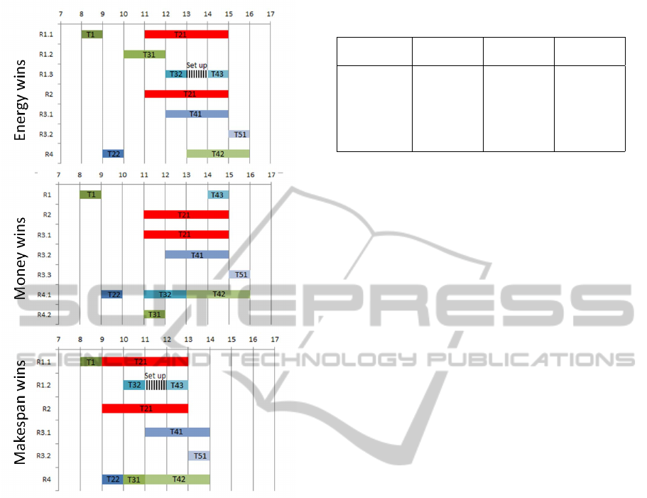
Figure 3: Resource assignment. Top: Energy wins sce-
nario. Centre: Money wins scenario. Bottom: Makespan
wins scenario.
since only one of the options of the XOR node would
actually be required to be executed, i.e. if task T21 is
performed, then the other tasks that R1 is allocated to
(T31, T32, and T43) will not be performed.
If we look at T21, we see how the bundles are
allocated differently in each of the scenarios. In the
energy priority scenario (top of Figure 3) T21 is as-
signed to R1 and R2 (at time 11), in the monetary
priority scenario T21 is assigned to R2 and R3 (also
at time 11), and in the makespan scenario T21 is as-
signed to R1 and R3 again, but at time 9. In the fig-
ure, it is possible to observe how parallel branches
(tasks T41 and T42) do not need to be executed at the
same time. Finally, note that set-up costs have only
been considered in the energy and makespan scenar-
ios, when sequencing tasks T32 and T43 in R1.
To quantify the results obtained, we have mea-
sured the worst (max) and best (min) cost on each sce-
nario. We have a range of possible costs for each sce-
nario because of the uncertainty associated with XOR
Table 3: Comparison of three scenarios (Cost
e
and Cost
e
are in Euros, whereas Cost
t
is in hours).
Scenario 1 Scenario 2 Scenario 3
Energy Money Makespan
Max Cost
e
11.58 15.38 12.28
Min Cost
e
2.84 3.97 3.02
Max Cost
e
1760.00 1320.00 1760.00
Min Cost
e
780.00 560.00 780.00
Max Cost
t
8.00 8.00 6.00
Min Cost
t
7.00 8.00 5.00
nodes: we don’t know in advance which branch will
be taken. The results obtained are shown in Table 3. If
we compare the worst case energy costs between sce-
narios 1 and 2, the energy cost in scenario 2 is 33%
more than scenario 1 (11.58 vs. 15.38). The monetary
cost in scenario 1 is 33.3% more than in scenario 2
(1760 vs. 1320). In the best case monetary cost sce-
nario, the difference in monetary cost between scenar-
ios 1 and 2 increases to 39% (780 vs. 560). However,
in this case scenario 1 has a lower makespan than sce-
nario 2. Money and energy are moving in different
scales (hundreds versus tens). However, with our ex-
periments we are showing how the resource selection
changes the energy costs. In other scenarios, energy
could be more expensive.
In the makespan scenario (scenario 3), the mon-
etary cost is the same as in scenario 1, however, the
energy cost increases by 6% both in the best and worst
case scenarios when compared to scenario 1. It should
be noted that resources are more idle in scenario 1
than scenario 2 (worst case make span of 8 vs. 6).
The results presented in Table 3 show three what-
if scenarios modelled, which can be valuable for deci-
sion makers (e.g. managers of the business processes).
They can use this information to consider trade-offs
between alternatives. For example, a manager cur-
rently employing the makespan strategy (scenario 3),
can now consider the trade-off in moving towards a
scenario where energy costs are minimised (i.e. sce-
nario 1).
5 DISCUSSION AND FUTURE
WORK
This paper presents an approach that considers energy
as one of the attributes for optimising resource alloca-
tions in business processes. Towards that end, this pa-
per presents the problem formalisation and discusses
an auction mechanism that can be employed. One of
the key contributions of this paper is the consideration
of time-dependent energy costs as a part of schedul-
ing and resource allocation, which has not been pre-
SMARTGREENS2014-3rdInternationalConferenceonSmartGridsandGreenITSystems
74

viously considered by work on BPM.
We used an auction mechanism to illustrate a pos-
sible instantiation of the problem formalisation and
different outcomes, depending on the cost focus: en-
ergy, price and makespan. They have been analyzed
using three what-if scenarios, to show how business
managers can consider the consequences of consider-
ing energy during the resource allocation process.
Considering energy as a key component in
scheduling and resourcing business process execu-
tions offers interesting challenges. For example, for
an organisation to adhere to the ISO norms of be-
ing energy efficient and also consuming green energy
(ISO, 2011), an organisation may choose to negotiate
a deal with the energy provider based on the energy
signature (or energy consumption shape curve) for
a particular day. Energy providers can offer special
rates for those companies that adhere to their expected
energy shape (i.e. energy usage at different hours of
the day).
This leads to other interesting scenarios such as
companies offering auctions on excess surplus en-
ergy to those that need some additional energy, simi-
lar to the dynamic coalition formation scenario con-
sidered for the construction of virtual power plants
(Mihailescu et al., 2011). One approach to address
this problem is to enable Workflow Management Sys-
tems (Ehrler et al., 2005) in charge of business pro-
cess resource allocations to coordinate their activities
with Energy Management Systems (EnMS) that are in
charge of company energy policy (Roche et al., 2010).
An EnMS can facilitate choosing external resources
that closely align with the energy objective functions
of a given organisation.
REFERENCES
Ardagna, D., Cappiello, C., Lovera, M., Pernici, B., and
Tanelli, M. (2008). Active energy-aware management
of business-process based applications. In Service-
Wave ’08, pages 183–195. Springer-Verlag.
Cappiello, C., Fugini, M., Gangadharan, G., Ferreira, A.,
Pernici, B., and Plebani, P. (2010). First-step toward
energy-aware adaptive business processes. In On the
Move to Meaningful Internet Systems: OTM 2010,
volume 6428 of LNCS, pages 6–7. Springer.
Chevaleyre, Y., Dunne, P. E., Endriss, U., Lang, J.,
Lema
ˆ
ıtre, M., Maudet, N., Padget, J., Phelps, S.,
Rodr
´
ıguez-Aguilar, J. A., and Sousa, P. (2006). Is-
sues in multiagent resource allocation. Informatica,
30:2006.
Chien, S. A., Tran, D., Rabideau, G., Schaffer, S. R., Mandl,
D., and Frye, S. (2010). Timeline-based space op-
erations scheduling with external constraints. In In-
ternational Conference on Automated Planning and
Scheduling (ICAPS), pages 34–41. AAAI.
Collins, J. and Gini, M. (2009). Scheduling tasks using
combinatorial auctions: the MAGNET approach. In
Adomavicius, G. and Gupta, A., editors, Business
Computing, volume 3 of Handbooks in Information
Systems, pages 263–294. Emerald.
Ehrler, L., Fleurke, M., Purvis, M., Tony, B., and
Savarimuthu, R. (2005). Agent based workflow man-
agement systems (WfMS): JBees - A distributed and
adaptive WfMS with monitoring and controlling ca-
pabilities. Journal of Information Systems and e-
Business Management, 4(1):5–23.
Gottwalt, S., Ketter, W., Block, C., Collins, J., and Wein-
hardt, C. (2011). Demand side management – A sim-
ulation of household behavior under variable prices.
Energy Policy, 39(12):8163–8174.
Hoesch-Klohe, K., Ghose, A., and L
ˆ
e, L.-S. (2010). To-
wards green business process management. In Pro-
ceedings of the IEEE International Conference on
Services Computing (SCC), pages 386–393.
ISO (2011). Energy management systems – require-
ments with guidance for use. ISO 50001:2011,
http://www.iso.org/iso/ (Accessed: 21.2.2012).
Mihailescu, R.-C., Vasiran, M., and Ossowski, S. (2011).
Dynamic coalition formation and adaptation for vir-
tual power stations in smart grids. In Int. Workshop
on Agent Technologies for Energy Systems (ATES).
Nowak, A., Leymann, F., and Schumm, D. (2011). The dif-
ferences and commonalities between green and con-
ventional business process management. In 2011
IEEE Ninth Int. Conf. on Dependable, Autonomic and
Secure Computing (DASC), pages 569 –576.
Parkes, D. C., Kalagnanam, J., and Eso, M. (2001).
Achieving budget-balance with Vickrey-based pay-
ment schemes in exchanges. In Int. Joint Conf. on
Artificial Intelligence (IJCAI), pages 1161–1168.
Ramchurn, S. D., Mezzetti, C., Giovannucci, A., Ro-
driguez, J. A., Dash, R. K., and Jennings, N. R.
(2009). Trust-based mechanisms for robust and ef-
ficient task allocation in the presence of execution un-
certainty. Journal of Artificial Intelligence Research,
35:119–159.
Roche, R., Blunier, B., Miraoui, A., Hilaire, V., and
Koukam, A. (2010). Multi-agent systems for grid en-
ergy management: A short review. In IECON 2010 -
36th Annual Conference on IEEE Industrial Electron-
ics Society, pages 3341–3346.
Simonis, H. and Hadzic, T. (2010). An energy cost aware
cumulative. In Third Int. Workshop on Bin Packing
and Placement Constraints (BPPC). 6 pages.
Syropoulos, A. (2001). Mathematics of multisets. In
Calude, C., Paun, G., Rozenberg, G., and Salomaa, A.,
editors, Multiset Processing: Mathematical,Computer
Science, and Molecular Computing Points of View,
volume 2235 of LNCS, pages 347–358. Springer.
TowardsEnergy-awareOptimisationofBusinessProcesses
75
