On Selecting Helpful Unlabeled Data for Improving Semi-Supervised
Support Vector Machines
∗
Le Thanh-Binh and Kim Sang-Woon
Department of Computer Engineering, Myongji University, Yongin, 449-728 South Korea
Keywords:
Semi-Supervised Learning, Support Vector Machines, Semi-Supervised Support Vector Machines.
Abstract:
Recent studies have demonstrated that Semi-Supervised Learning (SSL) approaches that use both labeled and
unlabeled data are more effective and robust than those that use only labeled data. However, it is also well
known that using unlabeled data is not always helpful in SSL algorithms. Thus, in order to select a small
amount of helpful unlabeled samples, various selection criteria have been proposed in the literature. One
criterion is based on the prediction by an ensemble classifier and the similarity between pairwise training
samples. However, because the criterion is only concerned with the distance information among the samples,
sometimes it does not work appropriately, particularly when the unlabeled samples are near the boundary. In
order to address this concern, a method of training semi-supervised support vector machines (S3VMs) using
selection criterion is investigated; this method is a modified version of that used in SemiBoost. In addition
to the quantities of the original criterion, using the estimated conditional class probability, the confidence
values of the unlabeled data are computed first. Then, some unlabeled samples that have higher confidences
are selected and, together with the labeled data, used for retraining the ensemble classifier. The experimental
results, obtained using artificial and real-life benchmark datasets, demonstrate that the proposed mechanism
can compensate for the shortcomings of the traditional S3VMs and, compared with previous approaches, can
achieve further improved results in terms of classification accuracy.
1 INTRODUCTION
In semi-supervised learning (SSL) approaches, a large
amount of unlabeled data (U), together with labeled
data (L), is used to build better classifiers. That is,
SSL exploits the samples of U in addition to the la-
beled counterparts in order to improve the perfor-
mance of a classification task, which leads to a perfor-
mance improvement in the supervised learning algo-
rithms with a multitude of unlabeled data. However, it
is also well known that using U is not always helpful
for SSL algorithms. In particular, it is not guaranteed
that adding U to the training data (T), i.e. T = L∪U,
leads to a situation in which the classification perfor-
mance can be improved (Ben-David, S. et al., 2008;
Lu, T., 2009; Zhu, X., 2006). Therefore, if more is
known about the confidence levels involved in clas-
sifying U, informative data could be chosen and in-
cluded easily when training base classifiers. Further-
more, if a large amount of unlabeled samples could be
∗
This work was supported by the National Research
Foundation of Korea funded by the Korean Government
(NRF-2012R1A1A2041661).
added to the training set, then the number of training
samples could be expanded effectively. Using large
and strong training samples may lead to creating a
strongly learned classifier.
From this perspective, in order to select a small
amount of helpful unlabeled data, various select-
ing techniques have been proposed in the litera-
ture, including the self-training (McClosky, D. et al.,
2008; Rosenberg, C. et al., 2005), co-training (Blum,
A. and Mitchell, T., 1998; Du, J. et al., 2011),
cluster-then-label (Singh, A. et al., 2008; Goldberg,
A. B. et al., 2009; Goldberg, A. B., 2010), sim-
ply recycled strategy in SemiBoost (Mallapragada,
P. K. et al., 2009), incrementally reinforced semi-
supervised MarginBoost (SSMB) (Le, T. -B. and
Kim, S. -W., 2012), and other criteria used in active
learning (AL) algorithms (Dagan, I. and Engelson, S.
P., 1995; Riccardi, G. and Hakkani-Tur, D., 2005;
Kuo, H. -K. J. and Goel, V., 2005; Leng, Y. et al.,
2013). For example, in SemiBoost, Mallapragada et
al. measured the pairwise similarity in order to guide
the selection of a subset of U for each iteration and
to assign (pseudo) labels to them. That is, they first
48
Le T. and Kim S..
On Selecting Helpful Unlabeled Data for Improving Semi-Supervised Support Vector Machines.
DOI: 10.5220/0004810500480059
In Proceedings of the 3rd International Conference on Pattern Recognition Applications and Methods (ICPRAM-2014), pages 48-59
ISBN: 978-989-758-018-5
Copyright
c
 2014 SCITEPRESS (Science and Technology Publications, Lda.)

computed the confidence of all U samples based on
the prediction made by an ensemble classifier and the
similarity among the samples of L∪U. Then, they se-
lected a few samples with higher confidence to retrain
the ensemble classifier together with L. The selecting-
and-training step was repeated for the number of iter-
ations or until a termination criterion was met.
On the other hand, support vector machines
(SVMs) (Vapnik, V., 1995) are considered to be
strong and successful classifiers in pattern recognition
(PR). Unlike traditional classification models, such
as Bayesian decision rules, SVMs minimize the up-
per bound of the generalization error by maximiz-
ing the margin between the separating hyperplane and
training data. Hence, SVMs are a distribution-free
model that can overcome the problems of poor sta-
tistical estimation and small sample sizes. SVMs also
achieve greater empirical accuracy and better gener-
alization capabilities than other standard supervised
classifiers. With regard to combining SVMs with SSL
strategies, numerous models use unlabeled samples
to improve the classification performance, including
semi-supervised support vector machines (S3VMs)
(Bennett, K. P. and Demiriz, A., 1998), transduc-
tive support vector machines (TSVMs) (Joachims,
T., 1999b), EM algorithms with generative mixture
models (Nigam, K. et al., 2000), Bayesian S3VMs
(Chakraborty, S., 2011), help-training (which is a
variant of the self-training) S3VMs (Adankon, M.
M. and Cheriet, M., 2011), hybrid S3VMs (Jiang, Z.
et al., 2013), and S3VM-us (semi-supervised support
vector machines with unlabeled instances selection)
(Li, Y. -F. and Zhou, Z. -H., 2011).
Among these combined approaches, the semi-
supervised support vector machines (S3VMs) (Ben-
nett, K. P. and Demiriz, A., 1998; Chapelle, O. et al.,
2006) and the transductive support vector machines
(TSVMs) (Joachims, T., 1999b) are the most popular
approaches for utilizing unlabeled data. In particular,
S3VMs are constructed using a mixture of L (training
set) and U (working set) data, where the objective is
to assign class labels to the working set. Therefore,
when the working set is empty, the S3VM becomes
the standard SVM model. In contrast, when the train-
ing set is empty, it becomes an unsupervised learn-
ing approach (Bennett, K. P. and Demiriz, A., 1998;
Joachims, T., 1999b). Consequently, when both the
training and working sets are not empty, SSL strate-
gies can be used. In this case, the information from
U can be helpful for the training process. More-
over, without labels, the cost of extracting U samples
may be lower than that of providing more L samples.
Therefore, S3VMs create a richness of opportunity
for many PR researchers.
The combination of helpfulU samples with L data
increases the likelihood of more accurate classifica-
tion; however, the determination of estimated labels
for U often leads to a fault. If this fails, the added
U samples with incorrect labels not only decrease the
accuracy of the classification but also increase the dif-
ficulty in choosing a decision function. From this
perspective, in order to complement the weakness of
S3VM, various techniques, such as SemiBoost (Mal-
lapragada, P. K. et al., 2009), conjugate function strat-
egy (Sun, S. and Shawe-Taylor, J., 2010), S3VM-us
(Li, Y. -F. and Zhou, Z. -H., 2011), incrementally re-
inforced selection strategy (Le, T. -B. and Kim, S. -
W., 2012), manifold-preservinggraph reduction (Sun,
S. et al., 2014), etc., have been proposed in the litera-
ture. In SemiBoost, for example, the confidence value
of x
i
∈ U is computed using two quantities, i.e. p
i
and
q
i
, which are measured using the pairwise similarity
between x
i
and other U and L samples. However,
when x
i
is near the boundary between two classes, the
value is computed using U only, without referring to
L. Consequently, the value might be inappropriate for
selecting helpful samples. In order to address prob-
lem, a modified technique that minimizes the errors
in estimating the labels of U is investigated.
This modification is motivated using the observa-
tion that, for samples x
i
∈U that are near the boundary
between the positive class of L (L
+
) and the negative
class of L (L
−
), three terms that comprise the selec-
tion criterion of SemiBoost are reduced to one term,
which only depends on U. That is, two of the three
terms, which are measured using L
+
and L
−
, respec-
tively, are changed to zero or nearly zero. From this
observation, the balance between the impacts of the
labeled and pseudo-labeled data is used when com-
puting the confidence values. The difference between
both criteria is two-fold: the first difference is that,
for the original criterion of SemiBoost, the confidence
values are computed using the quantities of p
i
and q
i
only, whereas for the modified criterion, they are mea-
sured using estimates of the conditional class proba-
bilities as well as the quantities of p
i
and q
i
. The sec-
ond difference is the method of labeling the selected
samples: in the original scheme, the label of x
i
∈ U is
predicted using a sign(p
i
− q
i
), while in the modified
scheme, this is predicted by referring to the probabil-
ity estimates as well as p
i
and q
i
.
The main contribution of this paper is the demon-
stration that the classification accuracy of S3VM can
be improved using a modified criterion when select-
ing unlabeled samples and predicting their labels.
Furthemore, a comparison of the classification per-
formance between the proposed S3VM and the tra-
ditional ones was performed empirically. In particu-
OnSelectingHelpfulUnlabeledDataforImprovingSemi-SupervisedSupportVectorMachines
49

lar, some critical questions concerning the strategies
employed in the present work were investigated, in-
cluding what are the features of the original S3VM
and SemiBoost that lead to the lower classification
accuracy? and why is the proposed modified criterion
better than the original?
The remainder of the paper is organized as fol-
lows. In Section 2, after providing a brief introduction
to S3VMs, an explanation for the use of selection cri-
terion in the SemiBoost algorithm is provided. Then,
in Section 3, a method of improving S3VMs through
utilizing the modified criterion for selecting a small
amount of helpful unlabeled samples is presented. In
Sections 4 and 5, the experimental setup and results
obtained using the experimental benchmark data are
presented, respectively. Finally, in Section 6, the con-
cluding remarks and limitations that deserve further
study are presented.
2 RELATED WORK
In this section, S3VM and SemiBoost, which are
closely related to the present empirical study, are
briefly reviewed. The details of the algorithms can
be found in the related literature (Vapnik, V., 1995;
Bennett, K. P. and Demiriz, A., 1998; Mallapragada,
P. K. et al., 2009).
2.1 S3VM and TSVM
A set of nl training pairs (L = {(x
1
,y
1
),··· ,(x
nl
,y
nl
)},
x
i
∈ R
d
, and y
i
∈ R) and a set of nu unlabeled sam-
ples (U = {x
1
,··· ,x
nu
} and x
j
∈ R
d
) are considered.
Referring to (Vapnik, V., 1995), SVMs have a de-
cision function f
θ
(·), which is defined as f
θ
(x) =
w· Φ(x) + b, where θ = (w,b) denotes the parameters
of the classifier model, w ∈ R
d
is a vector that de-
termines the orientation of the discriminating hyper-
plane, and b ∈ R is a bias constant such that b/kwk
represents the distance between the hyperplane and
origin. Also, Φ : R
d
→ F is a nonlinear feature map-
ping function, which is often implemented implicitly
using the kernel trick.
When denoting η
i
as the loss for x
i
, the quadratic
programming formulation is defined as follows:
min
1
2
kwk
2
+C
nl
∑
i=1
η
i
s.t. y
i
f
θ
(x
i
) + η
i
≥ 1,η
i
≥ 0,i = 1,··· ,nl,
(1)
where C > 0 is a fixed penalty regularization param-
eter, which is determined via trial and error (Vapnik,
V. and Chervonenkis, A. I., 1974), (Vapnik, V., 1982),
(Vapnik, V., 1995). In particular, S3VM is defined as
follows (Bennett, K. P. and Demiriz, A., 1998):
min
1
2
kwk
2
+C
nl
∑
i=1
η
i
+C
∗
nu
∑
j=1
η
j
s.t. y
i
f
θ
(x
i
) + η
i
≥ 1,i = 1,··· ,nl,
| f
θ
(x
j
)| ≥ 1− η
j
, j = 1,··· , nu.
(2)
S3VMs are an expansion of SVMs using an SSL
strategy, while TSVMs use the transductive learn-
ing approach. Given a set of nl training pairs (L)
and a (unlabeled) set of nt test samples in test set
(T
U
), the goal is to determine the pairs that an SVM
trained on L ∪ (T
U
×Y
∗
) can use to yield the largest
margin from the possible binary estimated label vec-
tors Y
∗
= (y
nl+1
,··· ,y
nl+nt
). This is a combinatorial
problem, but it can be approximated (see (Vapnik, V.,
1995)) to locating an SVM that separates the training
set under constraints, which forces the test unlabeled
samples to be as far as possible from the margin. This
can be written as follows:
min
1
2
kwk
2
+C
nl
∑
i=1
η
i
+C
∗
nt
∑
j=1
η
j
s.t. y
i
f
θ
(x
i
) + η
i
≥ 1,η
i
≥ 0,i = 1,··· ,nl,
| f
θ
(x
j
)| ≥ 1− η
j
, j = 1, · · · , nt.
(3)
This minimization problem is equivalent to mini-
mizing L, which is defined as follows:
L ≡
1
2
kwk
2
+ C
nl
∑
i=1
H
1
(y
i
f
θ
(x
i
)) (4)
+ C
∗
nt
∑
j=1
H
1
(| f
θ
(x
j
)|),
where H
1
(·) is the Hinge loss function defined as fol-
lows:
H
1
(γ) =

1− γ, if γ < 1
0 otherwise.
(5)
For C
∗
= 0 in (4), the standard SVM optimiza-
tion problem is obtained. For C
∗
> 0, the U data
that are inside the margin are penalized. This is
equivalent to using the Hinge loss on U as well, but
it is assumed that the label of the unlabeled exam-
ple x
i
is y
i
= sign( f
θ
(x
i
)). In order to solve (4),
Joachims (Joachims, T., 1999b) proposed an efficient
local search algorithm that is the basis of SVM
Light
(Joachims, T., 1999a).
2.2 SemiBoost
The goal of SemiBoost (Mallapragada, P. K. et al.,
2009), which is a boosting framework for SSL, is to
iteratively improve the performance of a supervised
ICPRAM2014-InternationalConferenceonPatternRecognitionApplicationsandMethods
50

learning algorithm (A) by regarding it as a black box,
using U and pairwise similarity. In order to follow
the boosting idea, SemiBoost optimizes performance
through minimizing the objective loss function de-
fined as follows (see Proposition 2 (Mallapragada, P.
K. et al., 2009)):
F
1
≤
nu
∑
i=1
(p
i
+ q
i
)(e
2α
+ e
−2α
− 1) (6)
−
nu
∑
i=1
2αh
i
(p
i
− q
i
),
where h
i
(= h(x
i
)) is the classifier learned by A at the
iteration, α is the weight for combining h
i
’s, and
p
i
=
nl
∑
j=1
S
ul
i, j
e
−2H
i
δ(y
j
,1) +
K
2
nu
∑
j=1
S
uu
i, j
e
H
j
−H
i
,
q
i
=
nl
∑
j=1
S
ul
i, j
e
2H
i
δ(y
j
,−1) +
K
2
nu
∑
j=1
S
uu
i, j
e
H
i
−H
j
.
(7)
Here, H
i
(= H(x
i
)) denotes the final combined
classifier and S denotes the pairwise similarity. For
all x
i
and x
j
of the training set, for example, S can be
computed using as follows:
S(i, j) = exp(−kx
i
− x
j
k
2
2
/σ
2
), (8)
where σ is the scale parameter controlling the
spread of the function. In addition, S
lu
(and S
uu
)
denotes the nl × nu (and nu × nu) submatrix of S.
Also, S
ul
and S
ll
can be defined correspondingly; the
constant K, which is computed using K = |L|/|U| =
nl/nu, is introduced to weight the importance be-
tween L and U; and δ(a,b) = 1 when a = b and 0
otherwise.
The quantities of p
i
and q
i
can be interpreted as
the confidence in classifying x
i
∈ U into a positive
class ({+1}) and negative class ({−1}), respectively.
Using these settings, p
i
and q
i
can be used to guide
the selection of U samples at each iteration using the
confidence measurement |p
i
− q
i
|, as well as to assign
the pseudo class label sign(p
i
− q
i
). The procedure
of selecting strong samples from U using confidence
levels, which is referred to as a sampling function, is
summarized as follows.
From (7), the difference in values between p
i
and
q
i
can be formulated as follows:
p
i
− q
i
=
nl
∑
j=1
S
ul
i, j
e
−2H
i
δ(y
j
,1)
−
nl
∑
j=1
S
ul
i, j
e
2H
i
δ(y
j
,−1)
+
C
2
nu
∑
j=1
S
uu
i, j
(e
H
j
−H
i
− e
H
i
−H
j
).
(9)
Algorithm 1: Sampling.
Input: Labeled data (L) and unlabeled data (U).
Output: Selected unlabeled data (U
s
).
Procedure: Repeat the following steps to select U
s
from U.
1. For each sample of U, compute classification con-
fidence levels ({|p
i
− q
i
|}
nu
i=1
) using (7).
2. After sorting the levels |p
i
− q
i
| in descending or-
der, choose a small portion from the top of the
unlabeled data (e.g. 10% top) as U
s
, according to
the confidence levels.
3. Update the estimated label for any selected sam-
ple x
i
by sign(p
i
− q
i
).
End Algorithm
By substituting L
+
≡ {(x
i
,y
i
)|y
i
= +1,i = 1,··· ,nl
+
}
and L
−
≡ {(x
i
,y
i
)|y
i
= −1,i = 1, · · · ,nl
−
} as the L
samples in class {+1} and class {−1}, respectively,
(9) can be represented as follows:
p
i
− q
i
=


e
−2H
i
∑
x
j
∈L
+
S
ul
i, j


−


e
2H
i
∑
x
j
∈L
−
S
ul
i, j


+
C
2
∑
x
j
∈U
S
uu
i, j
(e
H
j
−H
i
− e
H
i
−H
j
)
!
.
(10)
Again, by substituting X
+
i
≡ e
−2H
i
∑
x
j
∈L
+ S
ul
i, j
and
X
−
i
≡ e
2H
i
∑
x
j
∈L
− S
ul
i, j
in the first two corresponding
summations of the similarity distances from x
i
∈ U to
each x
j
∈ L in class {+1} and class {−1}, the differ-
ence in the values between X
+
i
and X
−
i
can be con-
sidered as the relative measurement for estimating the
possibility that x
i
belongs to {+1} or {−1} as fol-
lows:
X
+
i
− X
−
i
< 0 ⇒ P(x
i
∈ {+1}) < P(x
i
∈ {−1}),
X
+
i
− X
−
i
> 0 ⇒ P(x
i
∈ {+1}) > P(x
i
∈ {−1}).
(11)
From this representation, it can be seen that if the
difference of X
+
i
and X
−
i
is nearly zero, then the sam-
ple x
i
could remain on the boundary of the classi-
fier. Therefore, the classification of x
i
is a complicated
problem. In order to address this problem, SemiBoost
uses the third term in (10), which denotes the rela-
tive information (i.e. similarity) between x
i
∈ U and
x
j
∈ U. This may provide more meaningful informa-
tion for enlarging the margin.
However, providing more data is not always ben-
eficial. If the value obtained using the third term in
OnSelectingHelpfulUnlabeledDataforImprovingSemi-SupervisedSupportVectorMachines
51

(10) is very large or X
+
i
is nearly equal to X
−
i
, (10)
will generate some erroneous data. In that case, the
meaning achieved using the confidence of X
+
i
− X
−
i
may be lost and the estimation for x
i
will depend on
the U data. That is, the L samples do not affect the
estimation of x
i
label; therefore, the estimated label is
unsafe and untrustworthy.
3 PROPOSED METHOD
In this section, in order to overcome the above men-
tioned weakness, the selection/prediction criterion
based on p
i
and q
i
is modified and, using the modi-
fied criterion, a learning algorithm for S3VMs is pro-
posed.
3.1 Quadratic Optimization Problem
First, the focus is on optimizing (2) in order to mini-
mize the quadratic problem to improve the results of
S3VMs. Minimizing (2) leads to the generation of an
optimized classifier. Let the U
s
be a subset of ns sam-
ples selected from U that have a high possibility of
trust. That is, U is partitioned into two subsets, i.e.
the selected U and remaining U (U = U
s
∪U
r
), where
the cardinalities of U
s
and U
r
are ns and nr, respec-
tively. Thus, the minimum (2) would be divided into
two terms represented using brackets as follows:
min
1
2
kwk
2
+C
nl
∑
i=1
η
i
+
"
C
∗
ns
∑
j=1
η
j
+C
∗
nr
∑
k=1
η
k
#
s.t. y
i
f
θ
(x
i
) + η
i
≥ 1,η
i
≥ 0,i = 1,··· ,nl,
| f
θ
(x
j
)| ≥ 1− η
j
, j = 1,··· , nu.
(12)
Using the Hinge loss in (5) for TSVMs, min-
imizing (12) is similar to minimizing L, which is
computed as follows:
L =
1
2
kwk
2
+C
nl
∑
i=1
H
1
(y
i
f
θ
(x
i
))
+
"
C
∗
ns
∑
j=1
H
1
(| f
θ
(x
j
)|) +C
∗
nr
∑
k=1
H
1
(| f
θ
(x
k
)|)
#
.
(13)
From (13), it is easy to observe that a smaller value
can be achieved when reinforcing the training set with
U
s
and its predicted labels. Furthermore, by omitting
the term related to the U
r
subset from (13), the prob-
lem of minimizing L can be simplified to the mini-
mization of L
1
, which is defined as follows:
L
1
≡
1
2
kwk
2
+C
nl
∑
i=1
H
1
(y
i
f
θ
(x
i
))
+
"
C
∗
ns
∑
j=1
H
1
(| f
θ
(x
j
)|)
#
.
(14)
Thus, it can be seen that L
1
≤ L without losing
generality. From this observation, rather than opti-
mizing L , L
1
can be considered as a new quadratic
optimization problem. Furthermore, it should be
noted that the quadratic problem could be more ef-
ficiently optimized through the minimization of each
term in (14), not through a summation. Therefore,
a modified version of the selection criterion in (10)
could be considered. In subsequent sections, the
method of adjusting the selection (sampling) function
and using it are discussed.
3.2 Modified Criterion
As mentioned previously, using p
i
and q
i
can lead to
incorrect decisions in the selection and labeling steps;
this is particularly common when the summation of
the similarity measurement from x
i
∈ U to x
j
∈ L is
too weak, as follows:
X
+
i
− X
−
i
≪ X
u
i
, (15)
where X
u
i
≡

C
2
∑
x
j
∈U
S
uu
i, j
(e
H
j
−H
i
− e
H
i
−H
j
)

, or
X
+
i
≈ X
−
i
. (16)
In this situation, the confident measurement is formu-
lated as follows:
|p
i
− q
i
| ≃ |X
u
i
|. (17)
From (17), it can be observed that the confident
measurement of x
i
∈ U is computed using the distance
between x
i
and x
j
∈ U, while excluding L. As a conse-
quence, the measurement is determined using U only
and, therefore, sometimes it does not function as a cri-
terion for selecting strong samples. In order to avoid
this, the criterion of (10) can be improvedthrough bal-
ancing the three terms in (10), i.e. X
+
i
, X
−
i
, and X
u
i
.
This improvement can be achieved through balanc-
ing the three terms through a reduction in the impact
of the third term, especially when X
+
i
≈ X
−
i
. More
specifically, in order to reduce the impact, the condi-
tional class probability is estimated with each x
i
∈ U
in this paper. This idea is motivated from the rule of
mapping the selected unlabeled sample (x
i
) to a pre-
dicted label (y
i
) being viewed as a procedure for ob-
taining the estimates of a set of conditional probabili-
ties.
ICPRAM2014-InternationalConferenceonPatternRecognitionApplicationsandMethods
52

In order to obtain the estimates of the proba-
bilities, a method cited from the LIBSVM library
(Chang, C. -C. and Lin, C. -J., 2011) can be con-
sidered. Using the probability estimates as a penalty
cost, the criterion of (10), i.e. |p
i
− q
i
|, can be modi-
fied as follows:
|CL(x
i
)| =


X
+
i
− X
−
i
+ X
u
i
− (1− P
E
(x
i
))


, (18)
where P
E
(x
i
) denotes the probability estimates and
1− P
E
(x
i
) corresponds to the percentage of mistakes
when labeling x
i
. Using (18) as the criterion of select-
ing strong unlabeled samples, the sampling function
described in Section 2.2 can be modified as follows.
Algorithm 2: Modified Sampling.
Input: Labeled data (L) and unlabeled data (U).
Output: Selected unlabeled data (U
s
).
Procedure: Repeat the following steps to select U
s
from U.
1. For each sample of the available unlabeled
data, compute the classification confidence levels
{|CL(x
i
)|}
nu
i=1
using (18).
2. After sorting the levels in descending order,
choose a small portion of the top of the unlabeled
data (e.g. 10% top) as U
s
, according to their con-
fidence levels.
3. Update the estimated label for any selected sam-
ple x
i
using sign(CL(x
i
)).
End Algorithm
3.3 Proposed Algorithm
In this section, an algorithm that upgrades the con-
ventional S3VM through the modified criterion for
selecting helpful samples from U is presented. The
algorithm begins with predicting the labels of U us-
ing an SVM classifier trained with L only. After ini-
tializing the related parameters, e.g. the kernel func-
tion and its related conditions, the confidence levels
of U ({|CL(x
i
)|}
nu
i=1
) are calculated using (18). Then,
{|CL(x
i
)|}
nu
i=1
is sorted in descending order. After
selecting the samples ranked with the highest confi-
dence levels, combining them with L creates a train-
ing set for an S3VM classifier. In training the S3VM
classifier, the minimization problem, which corre-
sponds to (4), can be solved through minimization:
L
1
=
1
2
kwk
2
+C
nl
∑
i=1
H
1
(y
i
f
θ
(x
i
))
+C
∗
ns
∑
j=1
H
1
(sign(CL(x
i
)) f
θ
(x
j
)),
(19)
where H
1
is the Hinge loss function in (5).
Finally, the selection and training steps are re-
peated while verifying the training error rates of the
classifier. The repeated regression leads to an im-
proved classification process and, in turn, provides
better prediction of the labels over iterations. Con-
sequently, the best training set, which is composed of
L and U
s
samples, constitutes the final classifier for
the problem.
Based on this brief explanation, an algorithm for
improving the S3VM using the modified criterion is
summarized as follows, where the labeled and unla-
beled data (L and U), cardinality of U
s
, number of
iterations (e.g. t
1
= 100), and type of kernel function
and its related constants (i.e. C and C
∗
), are given as
input parameters. As outputs, the labels of all data
and the classifier model are obtained:
Algorithm 3: Proposed Algorithm.
Input: Labeled data (L) and unlabeled data (U).
Output: Final classifier (H
f
).
Method:
Initialization: Select U
(0)
s
from U through an SVM
trained with L; set the parameters, e.g. C and C
∗
, and
kernel function (Φ); train the first S3VM (H
f
) with
L∪U
(0)
s
and compute the training error (ε(H
f
)), using
L only.
Procedure: Repeat the following steps while increas-
ing i from 1 to t
1
in increments of 1.
1. Choose U
(i)
s
from U using the modified sampling
function (i.e., Algorithm 2), where the previously
trained S3VM is invoked.
2. Train a new S3VM classifier (h
i
) using both L and
U
(i)
s
, and obtain the training error (ε(h
i
)) with L.
3. If ε(h
i
) ≤ ε(H
f
), then keep h
i
as the best classifier,
i.e. H
f
← h
i
and ε(H
f
) ← ε(h
i
).
End Algorithm
The time complexities of the two algorithms, the
SemiBoost (Mallapragada, P. K. et al., 2009) algo-
rithm and the proposed algorithm, can be analyzed
and compared as follows. As in the case of Semi-
Boost algorithm, almost all the processing CPU-time
of the proposed algorithm is also consumed in com-
puting the three steps of Procedure in Algorithm 3.
So, the difference in magnitude between the compu-
tational complexities of SemiBoost and the proposed
algorithm depends on the computational costs associ-
ated with the routines of three steps. More specif-
ically, in both algorithms, the three steps are con-
cerned with: (1) sampling a small amount of the un-
labeled samples U using the criteria; (2) learning a
OnSelectingHelpfulUnlabeledDataforImprovingSemi-SupervisedSupportVectorMachines
53

Table 1: Comparison of time complexities of the three steps
for the SemiBoost algorithm and the proposed algorithm.
Here, | · | denotes the cardinality of a data set.
Steps SemiBoost algorithm Proposed algorithm
(1) Sampling O(|U| + |U|log|U|) O(|U| + |U|log|U|)
(2) Training O(|L| + |S|) O(|L| + |S|)
(3) Updating weights O(|L| + |U|) −
(and the best S3VM) O(1) O(1)
weak-learner (and S3VM in Algorithm 3) using the
labeled data L and the selected samples S; and (3) up-
dating the ensemble classifier with the appropriately
estimated weights for SemiBoost, while keeping the
best classifier for the proposed algorithm. From this
consideration, the time complexities for the steps can
be summarized in Table 1.
From Table 1, in the case of repeating the three
steps t times, the time complexities of the two algo-
rithms are, respectively, O(α
1
t) and O(α
2
t), where
α
1
= 2|U|+ |U|log|U|+2|L|+|S|+1and α
2
= |U|+
|U|log|U|+ |L|+ |S|+ 1, and, consequently, α
1
> α
2
.
From this analysis, it can be seen that the required
time for SemiBoost is much more sensitive to the car-
dinalities of the training sets (L and U) and the se-
lected data set (S) than that for the proposed algo-
rithm.
4 EXPERIMENTAL SETUP
In this section, in order to perform experiments for
evaluating the proposed approach, experimental data
and methods are described first.
4.1 Experimental Data
The proposed algorithm was evaluated and compared
with the traditional algorithms. This was accom-
plished through performing experiments on
the Image Classification Practical 2011 database
2
, which was published by Vedaldi and Zisserman
(Vedaldi, A. and Zisserman, A., 2011). This database
contains five groups of image data: person, horse,
car, aeroplane, and motorbike. Each group contains
one class {+1} and must be separated from the other
images, called the backgroundimage class {−1}. The
background images (1019/4000)are a different image
set that is not involved in the five groups mentioned
above. The qualification of all image sets is verified
using the PASCAL VOC’07 database (Everingham,
2
http://www.robots.ox.ac.uk/˜vgg/share/practical-image-
classification.htm
Table 2: Characteristics of the PASCAL VOC’07 database
used in the experiment. Here, four letter acronym, namely,
Aero, Moto, Pers, Car, Hors, and Back represent the Aero-
plane, Motorbike, Person, Car, Horse, and Background
groups, respectively.
Datasets Aero Moto Pers Car Hors Back
Object # 112 120 1025 376 139 1019
Feature # 4000 4000 4000 4000 4000 4000
M. et al., 2007). The characteristics for each group
are summarized in Table 2.
4.2 Experimental Methods
In this experiment, each dataset was divided into three
subsets, i.e. a labeled training set, labeled test set,
and unlabeled data set, with a ratio of 20%: 20%:
60%. The training and test procedures were repeated
ten times and the results were averaged. The (Gaus-
sian) radial basis function kernel, i.e. Φ(x,x
′
) =
exp(−(kx− x
′
k
2
2
)/2σ
2
), was used for all algorithms.
In the S3VM classifier, the two constants, C
∗
and
C, were set to 0.1 and 100, respectively, for sim-
plicity. The same scale parameter (σ), which was
found using cross-validation by training an inductive
SVM for the entire data set, was used for all meth-
ods. The proposed S3VM (hereafter referred to as
S3VM-improved) was compared with three types of
traditional SVMs, which were TSVM (Joachims, T.,
1999b), S3VM (Chang, C. -C. and Lin, C. -J., 2011),
and SemiBoost-SVM (SB-SVM) (Mallapragada, P.
K. et al., 2009), by selecting the top 10% from U.
5 EXPERIMENTAL RESULTS
The run-time characteristics of the proposed algo-
rithm are reported in the following subsections. Prior
to presenting the classification accuracies, the original
criterion and modified criterion are compared.
5.1 Comparison of Two Criteria:
Original and Modified
Prior to presenting the classification accuracies, the
original criterion and modified criterion were com-
pared. First, the following question was investigated:
does the modified selection criterion perform better
than the original criterion? To answer this question,
an experiment on selecting unlabeled samples fromU
was conducted using the original criterion in (9) and
the modified criterion in (18). The experiment was
ICPRAM2014-InternationalConferenceonPatternRecognitionApplicationsandMethods
54

−12 −10 −8 −6 −4 −2 0 2 4 6 8
−12
−10
−8
−6
−4
−2
0
2
4
6
8
(a)
−12 −10 −8 −6 −4 −2 0 2 4 6 8
−12
−10
−8
−6
−4
−2
0
2
4
6
8
(b)
4
3
2
1
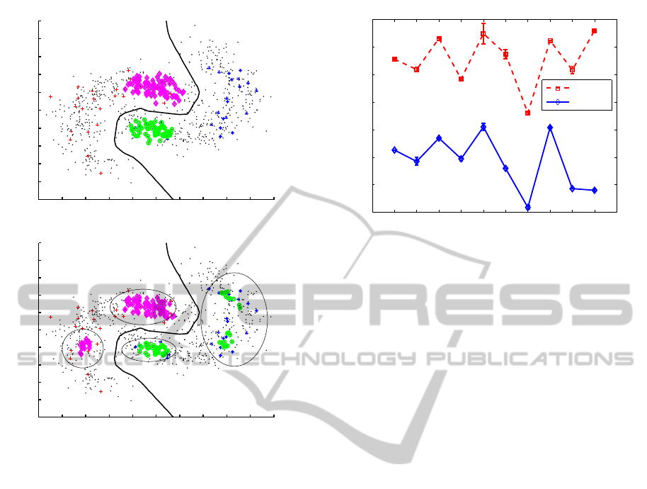
Figure 1: Plots comparing the selected samples with the
original criterion (a) and the modified criterion (b) for an
artificial dataset. Here, objects in the positive and negative
classes are denoted by ‘+’ and ‘∗’ symbols, respectively, in
different colors. The selected objects from the two classes
are marked with ‘⋄’ and ‘◦’ symbols, respectively from the
positive and negative classes, in different colors. The unla-
beled data are indicated using a ‘·’ symbol.
conducted as follows. First, two confidence values
were computed for all U samples with the two crite-
ria in (9) and (18). Second, a subset of U, i.e. U
s
(i.e. 10%), was selected referring to the confidence
values. Fig. 1 presents a comparison of the two se-
lections achieved using the above experiment for ar-
tificial data, which is a two-dimensional, two-class
dataset of [500,500] objects with a banana shaped
distribution (Duin,R. P. W. et al., 2004). The data
was uniformly distributed along the banana distribu-
tion and was superimposed with a normal distribution
with a standard deviationSD = 1 in all directions. The
class priorities are P(1) = P(2) = 0.5.
From the figure, it can be observed that the capa-
bility of selecting helpful samples for discrimination
is generally improved. This is clearly demonstrated
in the differences between Fig. 1 (a) and Fig. 1 (b)
in the number of selected samples and their geomet-
rical structures. More specifically, for the circled re-
10 20 30 40 50 60 70 80 90 100
0.08
0.1
0.12
0.14
0.16
0.18
0.2
0.22
The cardinality of the unlabeled subset (%)
Wrong prediction rates
Aeroplane
sign(p
i
− q
i
)
sign(CL(x
i
))
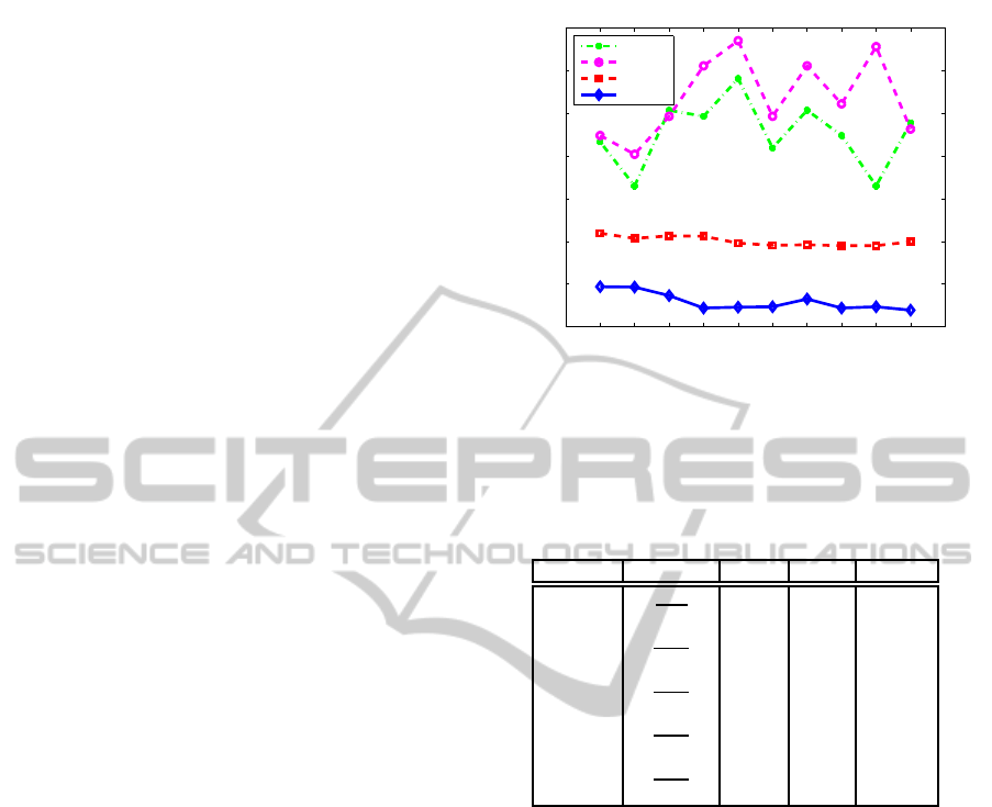
Figure 2: Comparison of the incorrect prediction rates be-
tween the original criterion and the modified criterion for
the experimental data.
gions #2 and #3, the number of selected points of the
modified criterion is smaller than that of the origi-
nal criterion. In contrast, for the regions #1 and #4,
the number of selected points for the modified crite-
rion is larger than that of the original criterion. In
the corresponding regions of the latter, there is no se-
lected point. From this observation, it should be noted
that the discriminative power of the modified criterion
might be better than that of the original criterion.
In order to further investigate this, another exper-
iment was conducted on labeling the unlabeled data
using the two selection criteria: a verification of the
two predicted labels for each x
i
∈ U using the two
criteria. The experiment was undertaken as follows.
First, a subset fromU (U
s
), for example, the 10% car-
dinality of U was randomly selected; second, the two
labels of all x
i
∈ U
s
predicted using the two techniques
in (9) and (18), i.e. sign(pi − qi) and sign(CL(xi)),
respectively, were compared with their true labels
(y
U
s
∈ {+1, −1}); these two steps were repeated af-
ter increasing the cardinality of U
s
by 10% until it
reached 100%. Fig. 2 presents a comparison of the
ten values obtained through repeating the above ex-
periment ten times for the Aeroplane dataset. In the
figure, the x-axis denotes the cardinality of U
s
and the
y-axis indicates the incorrect prediction rates obtained
using the two criteria.
From the figure, it can be observed that the pre-
diction capabilities of the original criterion and the
modified criterion generally differ from each other;
the capability of the modified criterion appears bet-
ter than that of the original criterion. This is clearly
demonstrated in the incorrect prediction rates of the
two criteria as represented by the dashed red line with
a  marker and the blue solid line with a ⋄ marker for
the original and modified criteria, respectively. For all
OnSelectingHelpfulUnlabeledDataforImprovingSemi-SupervisedSupportVectorMachines
55

the datasets and for each repetition, the lower rate was
always obtained with the modified criterion described
in (18), rather than the original criterion described in
(9). That is, in the comparison, the modified criterion
always obtained better performance (i.e. the red line
with the  marker is higher than the blue line with the
⋄ marker). The same characteristics can be observed
in the results from the other datasets. The results of
the other datasets are omitted here in order to avoid
repetition.
5.2 Comparison of Classification Error
Rates between Two Selection
Strategies
The following subsection investigates the classifica-
tion accuracy of the proposed algorithm, i.e. S3VM-
improved, using the modified criterion: is it better
(or more robust) than those of the traditional algo-
rithms when the number of selected samples is var-
ied? In order to answer this question and to assess
the accuracy of the two selection strategies in partic-
ular, the classification error rates of an SVM classi-
fier implemented with a polynomial kernel function
of degree 1 and a regularization parameter (C = 1),
but designed with different training sets (L and dif-
ferent U
s
subsets) were tested and evaluated. Here,
the two trained SVMs are the SemiBoost-SVM (SB-
SVM) and the proposed improved algorithm (S3VM-
improved). That is, the S3VM-improved uses the
modified criterion to select helpful samples, while the
SB-SVM uses the original criterion used in Semi-
Boost. The comparison was achieved by gradually
increasing the cardinality of U
s
from 0% to 100%.
A cardinality of 0% indicates that the SVM training
used only L, while that of 100% indicates that the
SVM training used the entire set of U in addition to
L. Fig. 3 presents the comparison of the classification
error rates of the two approaches for the Aeroplane
dataset. In the figure, the x-axis denotes the cardinal-
ity of U
s
to be added to L, while the y-axis indicates
the error rates obtained with the two S3VMs.
In Fig. 3, the blue solid line with a ⋄ maker
denotes the classification error rate of the S3VM-
improved, while the dashed lines with the ◦, ⊙,
and  makers represent those of the three traditional
S3VMs, respectively. From the figure, it can be ob-
served that the classification accuracies of the SVM
algorithms are improved by choosing helpful samples
from U when using both L and U. This is clearly
demonstrated in the figure where the error rates of the
S3VM-improved,indicated by the ⋄ marker,are lower
than those of the SB-SVM, denoted using the  sym-
bol, for all the U
s
cardinalities. From these observa-
10 20 30 40 50 60 70 80 90 100
0.05
0.06
0.07
0.08
0.09
0.1
0.11
0.12
The cardinality of the unlabeled subset (%)
Error rates
Aeroplane
TSVM
S3VM
SBSVM
S3VM−im
Figure 3: Comparison of the classification error rates of the
two algorithms for the experimental data.
Table 3: Numerical comparison of the classification er-
ror (and standard deviation) rates (%) between the S3VM-
improved and traditional algorithms for VOC’07 datasets.
Here, the lowest error rate in each data set is underlined.
Datasets S3VM-imp TSVM S3VM SB-SVM
Aeroplane 5.33 8.74 10.07 7.52
(0.44) (0.51) (0.93) (0.77)
Motorbike 10.00 17.18 17.18 10.96
(0.66) (2.02) (1.53) (0.64)
Person 31.75 41.28 43.84 37.80
(2.12) (3.99) (3.27) (2.52)
Car 18.13 22.46 24.51 19.12
(1.49) (2.30) (2.23) (1.29)
Horse 10.71 17.25 20.91 12.97
(1.05) (3.21) (2.32) (1.09)
tions, it can be determined that the proposed mech-
anism using the modified criterion works well with
semi-supervised SVMs.
5.3 Numerical Comparison of the Error
Rates
In order to further investigate the characteristics of the
proposed algorithm, the experiment was repeated us-
ing different VOC’07 datasets. Table 3 presents a nu-
merical comparison of the mean error rates and stan-
dard deviations obtained from the experiments. Here,
the results in the second column were obtained us-
ing the proposed S3VM-improved algorithm where
the cardinality of U
s
is 10%; the results of the third,
fourth, and fifth columns were obtained using the
TSVM, S3VM, and SB-SVM, which were imple-
mented using the algorithms provided in (Joachims,
T., 1999b), (Chang, C. -C. and Lin, C. -J., 2011), and
(Mallapragada, P. K. et al., 2009), respectively.
ICPRAM2014-InternationalConferenceonPatternRecognitionApplicationsandMethods
56

In addition to this result, in order to demonstrate
the significant differences in the error rates between
the S3VM algorithms used in the experiments, for the
means (µ) and standard deviations (σ) shown in Ta-
ble 3, the Student’s statistical two-sample test (Huber,
P. J., 1981) can be conducted. More specifically, us-
ing the t-test package, the p-value can be obtained in
order to determine the significance of the difference
between these algorithms. Here, the p-value repre-
sents the probability that the error rates of the S3VM-
improved algorithm are generally smaller than those
of the traditional S3VM algorithms.
For example, for the Motorbike dataset with
µ
1
(σ
1
) = 0.1000(0.0066) for the S3VM-improved al-
gorithm and µ
2
(σ
2
) = 0.1096(0.0064) for the SB-
SVM algorithm (refer to Table 3), a p-value of 0.998
was obtained for the two algorithms. As a conse-
quence, because p > 0.95 at the 5% significance level,
the null hypothesis H0: µ
1
(σ
1
) = µ
2
(σ
2
) was rejected
and the alternative hypothesis H1: µ
1
(σ
1
) < µ
2
(σ
2
)
was accepted. In a similar manner, it can be ob-
served that all Practical Image VOC’07 datasets per-
formed better at significant levels of both 5% and
10%. From this observation, it is clear that the er-
ror rate of S3VM-improved is smaller than those of
the traditional S3VM algorithms.
5.4 Comparison of the Time
Complexities
Finally, the time complexity of the proposed algo-
rithm for the VOC’07 data sets was investigated.
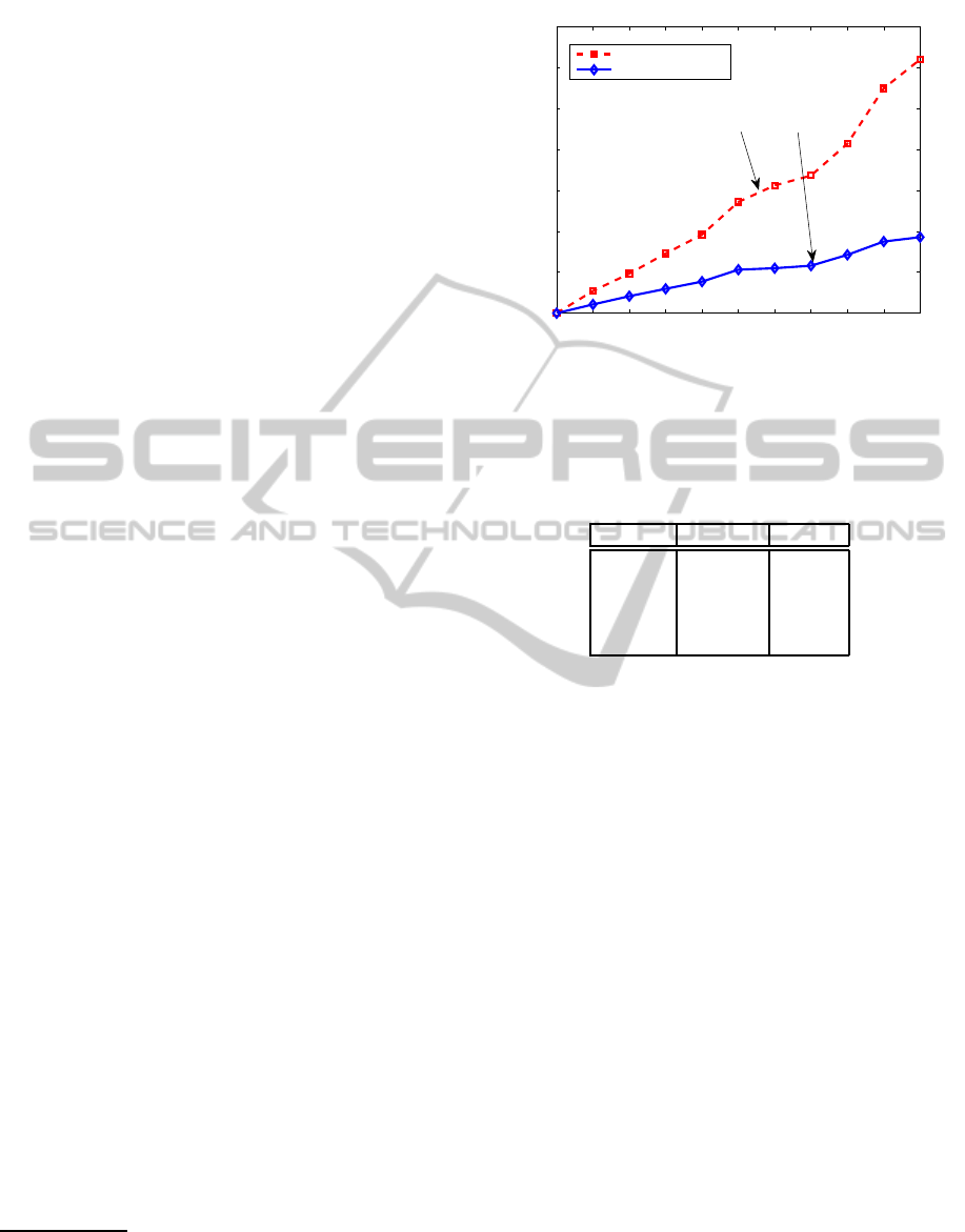
First, Fig. 4 presents a comparison of the process-
ing CPU-times (in seconds) obtained through repeat-
ing the above experiment ten times for the Aeroplane
dataset. In the figure, the x-axis denotes the number
of iterations (t) and the y-axis indicates the processing
CPU-times corrupted by the two algorithms.
From Fig. 4, as mentioned in Section 3.3, it can
be observed that the required time for SemiBoost is
much more sensitive to the cardinalities of the train-
ing sets (L and U) and the selected data set (S) than
that for the proposed algorithm. The details of the
other data sets are omitted here in the interest of com-
pactness.
Next, the processing CPU-times (in seconds)
3
of
the S3VM-imp and SB-SVM methods for the VOC’07
data sets are shown in Table 4.
From the results of the table, we can see a com-
parison of the results obtained with the S3VM-imp
3
The times recorded are the times required for the MAT-
LAB computation on a PC with a CPU speed of 2.8 GHz
and RAM 4096 MB, and operating on a Window 7 Enter-
prise 64-bit platform.
0 1 2 3 4 5 6 7 8 9 10
0
10
20
30
40
50
60
70
Aeroplane
# of iterations (t)
Processing CPU−times (sec)
SemiBoost (SB−SVM)
Proposed (S3VM−imp)
Slope: α
1
>
Slope: α
2
Figure 4: Comparison of the processing CPU-times (in sec-
onds) required for the training-test computation for the ex-
perimental data set.
Table 4: Numerical comparison of the processing CPU-
times (seconds) between the S3VM-improved and SB-SVM
algorithms for VOC’07 datasets.
Datasets S3VM-imp SB-SVM
Aeroplane 18.57 62.00
Motorbike 29.18 82.92
Person 178.42 444.10
Car 58.76 159.80
Horse 30.67 86.78
and SB-SVM for the VOC’07 data sets. From these
considerations, the reader should observe that the pro-
posed philosophy of S3VM-imp needs less time than
that of the traditional SB-SVM in the cases of the
VOC’07 data sets.
6 CONCLUSIONS
In an effort to improve the classification performance
of S3VM algorithms, selection criteria with which the
algorithms can be implemented efficiently were in-
vestigated in this paper. S3VMs are a popular ap-
proach that attempts to improve learning performance
through exploiting the whole or a subset of unlabeled
data. For example, in SemiBoost, a strategy of im-
proving the accuracy of the SVM classifier through
selecting a few helpful samples from the unlabeled
data has been proposed. However, the selection crite-
rion has a weakness that is caused by the significant
influence of the unlabeled data on the prediction of
the labeling for the selected samples. This impact can
cause errors in selecting and labeling unlabeled sam-
ples. In order to avoid this significant effect, the se-
lection criterion was modified using the conditional
OnSelectingHelpfulUnlabeledDataforImprovingSemi-SupervisedSupportVectorMachines
57

class probability estimated and the original quanti-
ties used for SemiBoost. This was motivated by an
observation that the confidence levels relating to the
unlabeled samples could be adjusted by subtracting
the probability estimates as a penalty cost. Using the
modified criterion, the confidence values relating to
the labeled and unlabeled data can be balanced.
The experimental results demonstrate that the
modified sampling criterion performs well with the
S3VM, particularly when the impacts of the positive
class and negative class are similar at the boundary.
Furthermore, the results demonstrate that the classifi-
cation accuracy of the proposed algorithm is superior
to that of the traditional algorithms when appropri-
ately selecting a small amount of unlabeled data. Al-
though it has been demonstrated that S3VM can be
improved using the modified criterion, many tasks re-
main to be improved. A significant task is the selec-
tion of an optimal, or near optimal, cardinality for the
strong samples in order to further improve the clas-
sification accuracy. Furthermore, it is not yet clear
which types of significant datasets are more suitable
for using the selection strategy for S3VM. Finally, the
proposed method has limitations in the details that
support its technical reliability, and the experiments
performed were limited. Future studies will address
these concerns.
REFERENCES
Adankon, M. M. and Cheriet, M. (2011). Help-training for
semi-supervised support vector machines. In Pattern
Recognition, volume 44, pages 2946–2957.
Ben-David, S., Lu, T., and Pal, D. (2008). Does unlabeled
data provably help? worst-case analysis of the sam-
ple complexity of semi-supervised learning. In Proc.
the 22th Ann. Conf. Computational Learning Theory
(COLT08), pages 33–44, Helsinki, Finland.
Bennett, K. P. and Demiriz, A. (1998). Semi-supervised
support vector machines. In Proc. Neural Information
Processing Systems, pages 368–374.
Blum, A. and Mitchell, T. (1998). Combining labeled and
unlabeled data with co-training. In Proc. the 11th Ann.
Conf. Computational Learning Theory (COLT98),
pages 92–100, Madison, WI.
Chakraborty, S. (2011). Bayesian semi-supervised learning
with support vector machine. In Statistical Methodol-
ogy, volume 8, pages 68–82.
Chang, C. -C. and Lin, C. -J. (2011). LIBSVM : a library for
support vector machines. In ACM Trans. on Intelligent
Systems and Technology, volume 2, pages 1–27.
Chapelle, O., Sch¨olkopf, B., and Zien, A. (2006). Semi-
Supervised Learning. The MIT Press, Cambridge,
MA.
Dagan, I. and Engelson, S. P. (1995). Committee-based
sampling for training probabilistic classifiers. In A.
Prieditis, S. J. Russell, editor, Proc. Int’l Conf. on Ma-
chine Learning, pages 150–157, Tahoe City, CA.
Du, J., Ling, C. X., and Zhou, Z. -H. (2011). When does co-
training work in real data? In IEEE Trans. on Knowl-
edge and Data Eng., volume 23, pages 788–799.
Duin,R. P. W., Juszczak, P., de Ridder, D., Paclik, P.,
Pekalska, E., and Tax, D. M. J. (2004). PRTools 4:
a Matlab Toolbox for Pattern Recognition. Delft Uni-
versity of Technology, The Netherlands.
Everingham, M., Van Gool, L., William, C. K. I., Winn,
J., and Zisserman, A. (2007). The PASCAL Visual
Object Classes Challenge 2007 (VOC2007) Results.
Goldberg, A. B. (2010). New Directions in Semi-Supervised
Learning. University of Wisconsin - Madison, Madi-
son, WI.
Goldberg, A. B., Zhu, X., Singh, A., Zhu, Z., and Nowak,
R. (2009). Multi-manifold semi-supervised learning.
In D. van Dyk, M. Welling, editor, Proc. the 12th Int’l
Conf. Artificial Intelligence and Statistics (AISTATS),
pages 99–106, Clearwater, FL.
Huber, P. J. (1981). Robust Statistics. John Wiley & Sons,
New York, NY.
Jiang, Z., Zhang, S., and Zeng, J. (2013). A hybrid gener-
ative/discriminative method for semi-supervised clas-
sification. In Knowledge-Based System, volume 37,
pages 137–145.
Joachims, T. (1999a). Making large-Scale SVM Learning
Practical. In B. Sch?lkopf, C. Burges, A. Smola, ed-
itor, Advances in Kernel Methods - Support Vector
Learning, pages 41–56, Cambridge, MA. The MIT
Press.
Joachims, T. (1999b). Transductive inference for text clas-
sification using support vector machines. In Proc. the
16th Int’l Conf. on Machine Learning, pages 200–209,
San Francisco, CA. Morgan Kaufmann.
Kuo, H. -K. J. and Goel, V. (2005). Active learning with
minimum expected error for spoken language under-
standing. In Proc. the 9th Euro. Conf. on Speech Com-
munication and Technology, pages 437–440, Lisbon.
Interspeech.
Le, T. -B. and Kim, S. -W. (2012). On improving semi-
supervised MarginBoost incrementally using strong
unlabeled data. In P. L. Carmona, J. S. S´anchez,
and A. Fred, editor, Proc. the 1st Int’l Conf. Pat-
tern Recognition Applications and Methods (ICPRAM
2012), pages 265–268, Vilamoura-Algarve, Portugal.
Leng, Y., Xu, X., and Qi, G. (2013). Combining active
learning and semi-supervised learning to construct
SVM classifier. In Knowledge-Based Systems, vol-
ume 44, pages 121–131.
Li, Y. -F. and Zhou, Z. -H. (2011). Improving semi-
supervised support vector machines through unlabeled
instances selection. In Proc. the 25th AAAI Conf. on
Artificial Intelligence (AAAI’11), pages 386–391, San
Francisco, CA.
Lu, T. (2009). Fundamental Limitations of Semi-Supervised
Learning. University of Waterloo, Waterloo, Canada.
Mallapragada, P. K., Jin, R., Jain, A. K., and Liu, Y. (2009).
SemiBoost: Boosting for semi-supervised learning. In
ICPRAM2014-InternationalConferenceonPatternRecognitionApplicationsandMethods
58

IEEE Trans. Pattern Anal. and Machine Intell., vol-
ume 31, pages 2000–2014.
McClosky, D., Charniak, E., and Johnson, M. (2008). When
is Self-Training Effective for Parsing? In Proc. the
22nd Int’l Conf. Computational Linguistics (Coling
2008), pages 561–568, Manchester, UK.
Nigam, K., McCallum, A. K., Thrun, S., and Mitchell, T.
(2000). Text classification from labeled and unla-
beled documents using EM. In Machine Learning,
volume 39, pages 103–134.
Riccardi, G. and Hakkani-Tur, D. (2005). Active learning:
theory and applications to automatic speech recogni-
tion. In IEEE Trans. on Speech and Audio Processing,
volume 13, pages 504–511.
Rosenberg, C., Hebert, M., and Schneiderman, H. (2005).
Semi-supervised self-training of object detection
models. In Proc. the 7th IEEE Workshop on Ap-
plications of Computer Vision / IEEE Workshop on
Motion and Video Computing (WACV/MOTION’05),
pages 29–36, Breckenridge, CO.
Singh, A., Nowak, R., and Zhu, X. (2008). Unlabeled data:
Now it helps, now it doesn’t. In T. Matsuyama, C.
Cipolla, et al., editor, Advances in Neural Information
Processing Systems (NIPS), pages 1513–1520, Lon-
don. The MIT Press.
Sun, S., Hussain, Z., and Shawe-Taylor, J. (2014).
Manifold-preserving graph reduction for sparse semi-
supervised learning. In Neurocomputing, volume 124,
pages 13–21.
Sun, S. and Shawe-Taylor, J. (2010). Sparse semi-
supervised learning using conjugate functions. In
Journal of Mach. Learn. Res., volume 11, pages
2423–2455.
Vapnik, V. (1982). Estimation of Dependencies Based on
Empirical Data (English translation 1982, Russian
version 1979.). Springer, New York.
Vapnik, V. (1995). The Nature of Statistical Learning The-
ory. Springer-Verlag, New York.
Vapnik, V. and Chervonenkis, A. I. (1974). Theory of Pat-
tern Recognition. Nauka, Moscow.
Vedaldi, A. and Zisserman, A. (2011). Image Classification
Practical, 2011.
Zhu, X. (2006). Semi-Supervised Learning Literature Sur-
vey. University of Wisconsin - Madison, Madison,
WI.
OnSelectingHelpfulUnlabeledDataforImprovingSemi-SupervisedSupportVectorMachines
59