
Self-adaptive Topology Neural Network for Online Incremental Learning
Beatriz P´erez-S´anchez, Oscar Fontenla-Romero and Bertha Guijarro-Berdi˜nas
Department of Computer Science, Faculty of Informatics, University of A Coru˜na,
Campus de Elvi˜na s/n, 15071, A Coru˜na, Spain
Keywords:
Incremental Learning, Sequential Learning, Forgetting Ability, Adaptive Topology, Vapnik-Chervonenkis
Dimension.
Abstract:
Many real problems in machine learning are of a dynamic nature. In those cases, the model used for the
learning process should work in real time and have the ability to act and react by itself, adjusting its control-
ling parameters, even its structures, depending on the requirements of the process. In a previous work, the
authors proposed an online learning method for two-layer feedforward neural networks that presents two main
characteristics. Firstly, it is effective in dynamic environments as well as in stationary contexts. Secondly, it
allows incorporating new hidden neurons during learning without losing the knowledge already acquired. In
this paper, we extended this previous algorithm including a mechanism to automatically adapt the network
topology in accordance with the needs of the learning process. This automatic estimation technique is based
on the Vapnik-Chervonenkis dimension. The theoretical basis for the method is given and its performance is
illustrated by means of its application to distint system identification problems. The results confirm that the
proposed method is able to check whether new hidden units should be added depending on the requirements
of the online learning process.
1 INTRODUCTION
In many applications, learning algorithms act in dy-
namic environments where data flows continuously.
In those situations, the algorithms should be able
to dynamically adjust to the underlying phenomenon
when new knowledge arrives. There are many learn-
ing methods and variants for neural networks. Classi-
cal batch learning algorithms are not suitable for han-
dling these types of situations. An appropriate ap-
proach would be an incremental learning technique
that assumes that the information available at any
given moment is incomplete and any learned theory
is potentially susceptible to changes. These types of
methods are able to adapt the previously induced con-
cept model during training. When dealing with neural
networks, this adaptation implies changing not only
the weights and biases but also the network architec-
ture. The adaptation of network topology depends on
the needs of the learning process, as the size of the
neural network should fit the number and complexity
of the data analyzed. The challenge is to find the cor-
rect network size, i.e., the smallest network structure
that allows reaching the desired performance specifi-
cations. If the network is too small it will not be able
to learn the problem well, but if its size is too large
it will lead to overfitting and poor generalization per-
formance (Kwok and Yeung, 1997). Therefore, the
network topology should be modified only if its ca-
pacities are insufficient to satisfy the needs of the pro-
cess of learning.
Different studies have proposed approaches that
modify the network topology as the learning process
evolves. Specifically there are two general strategies
to achieveit. The former trains a network that is larger
than necessary until an acceptable solution is found
and then removes hidden units and weights that are
not needed. The methods which follow this approach
are denominated pruning methods (Reed, 1993). In
the second approach the search for the suitable net-
work topology follows another direction, these are
the constructive algorithms (Bishop, 1995). These
methods start from a small network which later in-
creases its size, adding hidden units and weights, un-
til a satisfactory solution is found. Generally it is
considered that the pruning technique presents several
drawbacks with respect to the constructive approach
(Parekh et al., 2000).
An important aspect to consider is what is the ap-
propriate number of hidden units. This value is very
difficult to estimate theoretically; however, different
methods have been proposed to dynamically adapt the
94
Pérez-Sánchez B., Fontenla-Romero O. and Guijarro-Berdiñas B..
Self-adaptive Topology Neural Network for Online Incremental Learning.
DOI: 10.5220/0004811500940101
In Proceedings of the 6th International Conference on Agents and Artificial Intelligence (ICAART-2014), pages 94-101
ISBN: 978-989-758-015-4
Copyright
c
2014 SCITEPRESS (Science and Technology Publications, Lda.)

network structure during the learning process based
on several empirical measures. Among others, Ash
(Ash, 1989) developed an algorithm for the dynamic
creation of nodes where a new hidden neuron is gen-
erated when the training error rate is lower than a crit-
ical value.
Aylward and Anderson (Aylward and Anderson,
1991) proposed a set of rules based in the error rate,
the convergence criterion and the distance to the tar-
get error. Other studies researched the application
of evolutive algorithms to optimize the number of
hidden neurons and the value of the weights (Yao,
1999; Fiesler, 1994). Murata (Murata, 1994) studied
the problem of determinating the optimum number of
parameters from a statistical point of view. In (Ma
and Khorasani, 2003) new hidden units and layers
are included incrementally only when they are needed
based on monitoring the residual error that cannot be
reduced any further by the already existing network.
An approach referred to as error minimized extreme
learning machine that can add random hidden nodes
was included in (Islam et al., 2009). Despite the nu-
merous studies, the authors are not aware of an ef-
ficient method for determining the optimal network
architecture and nowadays this remains an open prob-
lem (Sharma and Chandra, 2010).
In a previous work (P´erez-S´anchez et al., 2013)
the authors presented an online learning algorithm
for two-layer feedforward neural networks, called
OANN, that includes a factor that weights the errors
committed in each of the samples. This method is ef-
fective in dynamic environments as well as in station-
ary contexts. This previous work also included the
study to check and justify the viability of OANN to
work with incremental data structures. In that study,
the modification of the topology is manually forced
every fixed number of iterations. In this paper, we ex-
tend the learning method by including an automatic
mechanism to check whether new hidden units should
be added depending on the requirements of the on-
line learning process. As a result, in this paper a
new learning algorithm denoted as automatic-OANN
is presented. This algorithm learns online and it is in-
cremental both with respect to its learning ability and
its topology.
The paper is structured as follows. In Section 2
the algorithm is explained. In Section 3, its behavior
is illustrated by its application to several time series
in order to check its performance in different con-
texts. In Section 4 the results are discussed and some
conclusions are given. Finally, in Section 5 we raise
some future lines of research.
2 DESCRIPTION OF THE
PROPOSED METHOD
To address the development of an automatic incre-
mental topology two crucial problems have to be
solved. First, there is a need to verify whether a learn-
ing algorithm can adapt the network topology by in-
corporating new hidden neurons while maintaining,
as much as possible, the knowledge gained in previ-
ous stages of learning.This challenge was solved in a
previous paper (P´erez-S´anchez et al., 2013) resulting
in OANN, which is summarized in section 2.1. Sec-
ondly, we must developed a mechanism to knowwhen
it is appropriate to change the network topology. This
is a new contribution that will be explained in sec-
tion 2.2. As a result, the new algorithm, automatic-
OANN, will be obtained.
2.1 How to Modify the Structure of the
Network
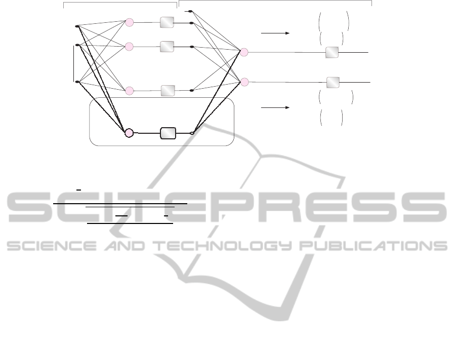
Consider the two-layer feedforward neural network in
Figure 1 where the inputs are represented as the col-
umn vector x(s), the bias has been included by adding
a constant input x
0
= 1, and outputs are denoted as
y(s), s = 1, 2, . . . , S where S is the number of training
samples. J and K are the number of outputs and hid-
den neurons, respectively. Functions g
1
, . . . , g
K
and
f
1
, . . . , f
J
are the nonlinear activation functions of the
hidden and output layer, respectively.
.
.
.
x
+
+
+
g
1
g
2
g
K
.
.
.
.
.
.
z
1
z
2
z
K
+
+
f
1
f
J
.
.
.
.
.
.
z
1
z
2
z
K
w
k
(1)
w
j
(2)
d
1
d
J
y
z
0
=1
subnetwork
1
subnetwork
2
.
.
.
x
0
=1
Figure 1: Two-layer feedforward neural network.
This network can be considered as the composi-
tion of two one-layer subnetworks. As the desired
outputs for each hidden neuron k at the current learn-
ing epoch s, z
k
(s), are unknown, arbitrary values are
employed. These values are obtained in base to a pre-
vious initialization of the weights using a standard
method, for example Nguyen-Widrow (Nguyen and
Widrow, 1990). The desired output of hidden nodes
are not revised during the learning process and they
are not influenced by the desired output of the whole
network. Thus, the training of the first subnetwork
is avoided in the learning task. Regarding the sec-
ond subnetwork, as d
j
(s) is the desired output for the
j output neuron, that it is always available in a su-
Self-adaptiveTopologyNeuralNetworkforOnlineIncrementalLearning
95

pervised learning, we can use
¯
d
j
(s) = f
−1
j
(d
j
(s)) to
define the objective function for the j output of sub-
network 2 as the sum of squared errors before the non-
linear activation function f
j
,
Q
(2)
j
(s) =
h
j
(s)
f
′
j
(
¯
d
j
(s))
w
(2)
j
T
(s)z(s) −
¯
d
j
(s)
2
(1)
where j = 1, . . . , J, w
(2)
j
(s) is the input vector of
weights for output neuron j at the instant s and
f
′
j
(
¯
d
j
(s)) is a scaling term which weighs the errors
(Fontenla-Romero et al., 2010). Moreover, the term
h
j
(s) is included as forgetting function and it deter-
mines the importance of the error at the s
th
sample.
This functionestablishes the form and the speed of the
adaptation to the recent samples in a dynamic context
(Mart´ınez-Rego et al., 2011).
The objective function presented in equation 1 is
a convex function, whose global optimum can be eas-
ily obtained deriving it with respect to the parame-
ters of the network and setting the derivative to zero
(Fontenla-Romero et al., 2010). Therefore, we obtain
the following system of linear equations,
K
∑
k=0
A
(2)
qk
(s)w
(2)
jk
(s) = b
(2)
qj
(s),
q = 0, 1, . . . , K; j = 1, . . . , J,
(2)
where
A
(2)
qk
(s) = A
(2)
qk
(s− 1) + h
j
(s)z
k
(s)z
q
(s) f
′
2
j
(
¯
d
j
(s)) (3)
b
(2)
qj
(s) = b
(2)
qj
(s− 1) + h
j
(s)
¯
d
j
(s)z
q
(s) f
′
2
j
(
¯
d
j
(s)) (4)
A
(2)
(s−1) and b
(2)
(s−1) being, respectively, the ma-
trices and the vectors that store the coefficients of the
system of linear equations employed to calculate the
values of the weights of the second layer in previ-
ous learning stage. In other words, the coefficients
employed to calculate the weights in the actual stage
are used further to obtain the weights in the follow-
ing one. Therefore, this permits handling the earlier
knowledge and using it to incrementally approach the
optimum value of the weights. Equation 2 can be
rewritten using matrix notation as,
A
(2)
j
(s)w
(2)
j
(s) = b
(2)
j
(s), j = 1, . . . , J,
(5)
where
A
(2)
j
(s) = A
(2)
j
(s− 1) + h
j
(s)z(s)z
T
(s) f
′
2
j
(
¯
d
j
(s))
b
(2)
j
(s) = b
(2)
j
(s− 1) + h
j
(s) f
−1
j
(d
j
(s))z(s) f
′
2
j
(
¯
d
j
(s))
Finally, from equation 3 the optimal weights for the
second subnetwork can be obtained as:
w
(2)
j
(s) = A
(2)
j
−1
(s)b
(2)
j
(s), ∀ j (6)
As regards the incremental property of the learn-
ing algorithm, the network structure can be adapted
depending on the requirements of the learning pro-
cess. Several modifications have to be carried out in
order to adapt the current topology to a new one. As
can be observed in Figure 2 the increment of hidden
neurons affects not only the first subnetwork (its num-
ber of output units increases) but also the second sub-
network (the number of its inputs also grows). As
mentioned previously, the training of the first subnet-
work is avoided in the training task, therefore we only
comment on the modifications corresponding to the
second subnetwork. Thus, in Figure 2 it can be ob-
served that as the number of hidden neurons grows
and consequently, all matrices A
(2)
j
and the vectors
b
(2)
j
(j = 1, . . . , J), computed previously modify their
size. Therefore in order to adapt them, each matrix
A
(2)
j
is enlarged by including a new row and a new
column of zero values, in order to continue the learn-
ing process from this point (zero is the null element
for the addition). At the same time, each vector b
(2)
j
incorporates a new element of zero value. The rest of
elements of the matrices and vectors are maintained
without variation, this fact allows us to preserve in
some way the knowledgeacquired previously with the
earlier topology. After these modifications, the latter
described matrices and vectors of coefficients allow
us to obtain the new set of weights for the current
topology of the network.
2.2 When to Change the Structure of
the Network
In statistical learning theory the Vapnik-Chervonenkis
dimension (Vapnik, 1998) is a measure of the capacity
of a statistical classification algorithm and it is defined
as the cardinality of the largest set of points that the
algorithm can shatter. Therefore, this term allows us
to predict a probabilistic upper bound on the test error
of a classification model based in its complexity. This
is an ideal bound that can be calculated according to
the training error and the network topology. If the
model generalizes properly, the bound indicates the
worst test error that the model can obtain. Thus, the
bound value establishes the margin to test error and
therefore it is possible to use this value to determine
whether the current topology is sufficient. In this way,
it can be said that an adequate number of hidden units
is the one giving the lowest expected risk. Taking into
account all these considerations it is established that,
with a probability of 1 − η the smallest test error (R,
expected risk) is delimited by the following inequality
(Vapnik, 1998),
ICAART2014-InternationalConferenceonAgentsandArtificialIntelligence
96
.
.
.
x
+
+
+
g
1
g
2
g
K
+
+
f
1
f
J
.
.
.
.
.
.
g
K+1
+
subnetwork
1
subnetwork
2
A
1
(2)
(s)
new hidden unit K+1
A
J
(2)
(s)
A
1
(2 )
(s) 0
0 0
b
1
(2)
(s)
b
1
(2)
(s)
0
A
J
(2 )
(s) 0
0 0
b
J
(2)
(s)
b
J
(2)
(s)
0
A
1
(1)
,
b
1
(1)
A
2
(1)
,
b
2
(1)
A
K
(1)
,
b
K
(1)
A
K+1
(1)
= 0
(I+1)x(I+1)
b
K+1
(1)
=
0
(I+1)x1
y
new
hidden
unit
.
.
.
.
.
.
new
hidden
unit
.
.
.
w
K+1
(1)
b
J
(2)
(s+1)=
A
J
(2)
(s+1)=
A
1
(2)
(s+1)=
b
1
(2)
(s+1)=
z
0
=1
z
1
z
2
z
K
x
0
=1
Figure 2: Incremental Topology.
R(d
VC
, θ) ≤
1
n
n
∑
i=1
(z
i
− ˆz
i
(d
VC
, θ))
2
1−
r
d
VC
ln
n
d
VC
+1
−ln
(
η
4
)
n
+
(7)
d
VC
represents the Vapnik-Chervonenkis dimension,
θ the ajustable parameters of the learning system, n
the number of training patterns, z target outputs, ˆz the
outputs obtained by the learning system and the no-
tation [.]
+
indicates the maximum value between 0
and the term between square brackets. It can be ob-
served that the numerator of equation 7 is the training
error and the denominator corresponds with a correc-
tion function.
In an informal way, we can say that the gener-
alization ability of a classification model is related
with the complexity of the structure. Specifically the
greater complexity, the greater value of the Vapnik-
Chervonenkis dimension and the lesser generalization
ability. In (Baum and Haussler, 1989), authors estab-
lished certain bounds to a particular network architec-
ture. Theyindicated an upper bound for a feedforward
neural network with M units (M ≥ 2) and W weights
(biases included) that allows to calculate the d
VC
vari-
able as
d
VC
≤ 2Wlog
2
(eM), (8)
e being the basis of the natural numbers. Although
equation 8 established an upper bound for the value
of the Vapnik-Chervonenkis dimension, this is a valid
approach as it allows calculating the error bound in
the worst case.
Taking into account all these considerations, an
automatic technique is developed to control the neural
network growth in the online learning algorithm. The
estimation method is based in the ideal bound for the
test error calculated thanks to Vapnik-Chervonenkis
dimension of the neural network. We obtained a con-
structive algorithm which adds a new unit to the hid-
den layer of the network when the obtained error test
is higher than the limit established by the ideal bound
(equation 8). Finally the new proposed online learn-
ing algorithm with incremental topology is detailed in
Algorithm 1.
3 EXPERIMENTAL RESULTS
In (P´erez-S´anchez et al., 2013), the OANN was com-
pared to other online algorithms and proved its suit-
ability to work with adaptive structures without sig-
nificantly degrading its performance. However, the
modification of the topology is manually forced every
fixed number of iterations. In this paper, we complete
the method with an automatic mechanism to control
whether new hidden units should be added depend-
ing on the requirements of learning process. In this
experimental study we want to demonstrate the via-
bility of the automatic adjustment mechanism of the
structure. Therefore, taking these results into account,
automatic-OANN will only be compared to the previ-
ous OANN version (fixed topology) with the follow-
ing objectives:
• To check if automatic-OANN is able to incorpo-
rate hidden units without significant performance
degradation with respect to the version without
adaptation of the topology.
• To prove that the performance of the automatic-
OANN at the end of the learning process, (when it
reaches a final network topology), is similar to the
performance that would be obtained by employing
this final topology from the beginning to the end
of learning process.
For this experimental study, we employed distinct
system identification problems. Moreover, the behav-
Self-adaptiveTopologyNeuralNetworkforOnlineIncrementalLearning
97

Algorithm 1: Automatic-OANN algorithm with adaptive
topology for two-layer feedforward neural networks.
Inputs: x
s
= (x
1s
, x
2s
, . . . x
Is
);d
s
= (d
1s
, d
2s
, . . . d
Js
); s = 1, . .. , S.
Initialization Phase
K = 2, initially the network has two units in its hidden
layer
A
(2)
j
(0) = 0
(K+1)×(K+1)
, b
(2)
j
(0) = 0
(K+1)
, ∀ j =
1, . . ., J.
Calculate the initial weights, w
(1)
k
(0), by means of an ini-
tialization method.
For every new sample s (s = 1, 2, . . . , S) and ∀k = 1, . . . , K
z
k
(s) = g(w
(1)
k
(0), x(s))
For each output j of the subnetwork 2 (j = 1, . . . , J),
A
(2)
j
(s) = A
(2)
j
(s− 1) + h
j
(s)z(s)z
T
(s) f
′
2
j
(
¯
d
j
(s)),
b
(2)
j
(s) = b
(2)
j
(s− 1) + h
j
(s) f
−1
j
(d
j
(s))z(s) f
′
2
j
(
¯
d
j
(s)),
Calculate w
(2)
j
(s) according to w
(2)
j
(s) =
A
(2)
j
−1
(s)b
(2)
j
(s)
end of For
Calculate Vapnik-Chervonenkis dimension, d
VC
, using
equation 8
Calculate the error test, MSE
Test
Calculate the test error bound using equation 7
If MSE
Test
> bound then a new hidden unit K+1 is added
A
(2)
j
(s) =
(K + 1)
A
(2)
j
(s− 1) 0 . . . 0 0
0 0 . . . 0 0
.
.
.
.
.
.
.
.
.
.
.
.
.
.
.
(K + 1) 0 0 . . . 0 0
0 0 . . . 0 0
,
b
(2)
j
(s) =
b
(2)
j
(s− 1)
0
(K + 1)
.
.
.
0
,
For each new connection,
calculate the weights, w
(1)
K+1
(0), by means of some ini-
tialization method
end of For
K = K + 1
end of If,
end of For
ior of the learning algorithm will be checked when
it operates in both stationary and dynamic environ-
ments. All experiments shared the following condi-
tions:
• In all cases, the logistic sigmoid function was em-
ployed for hidden neurons, while for output units
a linear function was applied as recommended for
regression problems (Bishop, 1995).
• The input data set was normalized, with mean=0
and standard deviation=1.
• In order to obtain significant results, five simula-
tions were carried out. Therefore, mean results
will be presented in this section. Moreover, in the
case of stationary context 10-fold cross validation
was applied.
• In all cases an exponential forgetting function, de-
fined as,
h(s) = e
µs
, s = 1, . . . , S, (9)
was employed, where µ is a positive real param-
eter that controls the growth of the function and
thus the response of the network to changes in the
environment. When µ = 0 we obtain a constant
function, and therefore all errors have the same
weight and the forgetting function has no effect.
The value of the µ factor for the forgetting ability
was set to 0.01.
3.1 Stationary Contexts
In this section, we consider two stationary time
series, H´enon and Mackey-Glass. The goal is to
predict the actual sample based in seven previous
patterns, in the case of H´enon series and according to
the eight previous pattern for Mackey-Glass. A brief
explanation of both time series is given as follow.
• H
´
enon. The H´enon map is a dynamic system that
presents a chaotic behavior (H´enon, 1976). The
map takes a point (x
n
, y
n
) in the plane and trans-
forms it according to,
x(t + 1) = y(t + 1) − αx(t)
2
y(t + 1) = γx(t)
x(t) being the series value at instant t. In this case
the parameters values are established as α = 1.4
and γ = 0.3. A total number of 4,000 patterns are
generated, 3,000 of them are used as training data
set and 1,000 patterns are employed to validate
the model.
• Mackey-Glass. The second example is the time
series of Mackey-Glass, which is generated due
to a system with a time delay difference as follows
(Mackey and Glass, 1977),
dx
dt
= βx(t) +
αx(t − γ)
1+ x(t − γ)
10
ICAART2014-InternationalConferenceonAgentsandArtificialIntelligence
98
x(t) being the value of the time series at the in-
stant t. The system is chaotic to gamma values
γ > 16.8. In this case, the series is generated
with the following parameters values α = 0.2, β =
−0.1, γ = 17 and it is scaled between [-1,1]. 3,000
samples are generated, 2,250 of them are selected
by training and 750 patterns are employed to eval-
uate the model.
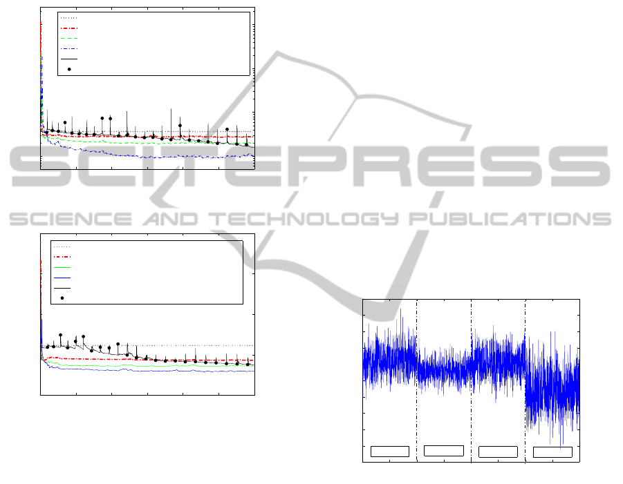
0 500 1000 1500 2000 2500 3000
10
−2
10
−1
10
0
10
1
sample/iteration
MSE
Fixed topolgy, 2 hidden units
Fixed topology, 8 hidden units
Fixed topology, 15 hidden units
Fixed topology, 27 hidden units
Incremental topology (from 2 to 27 hidden units)
Topology changes
Figure 3: Test error curves for the H´enon time series.
0 500 1000 1500 2000 2500 3000
10
−4
10
−2
10
0
10
2
10
4
sample/iteration
MSE
Fixed topology, 2 hidden units
Fixed topology, 8 hidden units
Fixed topology, 14 hidden units
Fixed topology, 25 hidden units
Incremental topology (from 2 to 25 hidden units)
Topology changes
Figure 4: Test error curves for the Mackey-Glass time se-
ries.
Figures 3 and 4 show the test MSE curves. In the
case of fixed topologies, curves are included for dif-
ferent number of hidden neurons. For readability only
the most significant results are shown. As can be ob-
served, the incremental topology algorithm achieves
results close to those obtained when the final fixed
topology is used from the initial epoch. The results
are not exactly the same but it should be considered
that the proposed method constructs the topology in
an online learning scenario and then only a few sam-
ples are available to train the last topology. The points
over the curves of incremental topology allow us to
know when the error obtained by the network exceeds
the bound established for the test error. At that mo-
ment, the structure is modified in order to response to
needs of the learning process.
3.2 Dynamic Environments
In dynamic environments, the distribution of the data
could change over time. Moreover, in these types
of environments, changes between contexts can be
abrupt when the distribution changes quickly or grad-
ual if there is a smooth transition between distribu-
tions (Gama et al., 2004). In order to check the perfor-
mance of the proposed method in different situations
we have considered both types of changing environ-
ments. The aim of these experiments is to check that
the proposed method is able to obtain appropriate be-
havior when it works in dynamic environments.
3.2.1 Artificial Data Set 1
The first data set is formed by 2,400 samples of 4
input random variables which contain values drawn
from a normal distribution with zero mean and stan-
dard deviation equal to 0.1. To obtain the desired out-
put, first, every input is transformed by a nonlinear
function. Specifically, hyperbolic tangent sigmoid,
exponential, sine and logarithmic sigmoid functions
were applied, respectively, to the first, second, third
and fourth output. Finally, the desired output is ob-
tained by a linear mixture of the transformed inputs.
0 300 600 900 1200 1500 1800 2100 2400
4.6
4.7
4.8
4.9
5
5.1
5.2
5.3
5.4
5.5
5.6
Sample
Desired output
context 4
context 3
context 2
context 1
Figure 5: Artificial Data Set 1. Example of the desired out-
put for the training set.
Figure 5 contains the signal employed as desired
target during the training process. As can be seen, the
signal evolves over time and 4 context changes are
generated. Also we created different test sets for each
context, so every training sample has associated the
test set that represents the context to which it belongs.
Thus, for this case we obtain 4 test sets, one for each
of the changes in the linear mixture of the process.
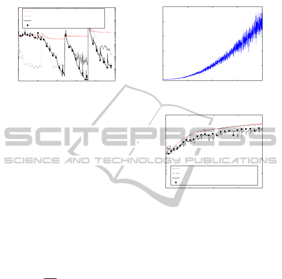
Figure 6 shows the test error curves obtained
by the method with fixed and automatic incremental
topologies. The error shown for each point of the sig-
nal is the mean value obtained over test set associated
to the current training sample. It can be seen that the
Self-adaptiveTopologyNeuralNetworkforOnlineIncrementalLearning
99
0 500 1000 1500 2000 2500
10
−6
10
−5
10
−4
10
−3
10
−2
10
−1
10
0
sample/iteration
MSE
Initial fixed topology (2 hidden units)
Final fixed topology (32 hidden units)
Incremental topology (from 2 to 32 hidden units)
Topology changes
Figure 6: Artificial Data Set 1: Test error curves.
initial fixed topology (two hidden neurons) commits
a high error because the structure is not sufficient to
make a suitable learning. Regarding the incremen-
tal topology, although the results at the beginning of
the process are not appropriate (the topology is still
small), it can be observed as it performs better than
the final fixed topology when there are changes of
context.
3.2.2 Artificial Data Set 2
In this case, we generated another artificial data set
that presents a gradual evolution in each sample of
training. The data set is formed by 4 input variables
(generated by a normal distribution with zero mean
and standard deviation equal to 0.1) and the output is
obtained by means of a linear mixture of these. In
order to construct the time series we fixed the initial
coefficients of the linear mixture vector as
a(0) =
0.5 0.2 0.7 0.8
, (10)
and subsequently these values evolve over time ac-
cording to the following equation,
a
j
(s) = a
j
(s−1)+
s
10
4.7
logsig(a
j
(s−1)), s = 1, . . . , S
where j indicates the component of the mixture vec-
tor. Finally, we obtained a set with S equals to 500
training samples. The signal employed as desired out-
put during the training process can be observed in Fig-
ure 7. As the distribution presents constant changes
we have a different context for each sample thus we
have a different test data set for each one.
Figure 8 shows the test error curves obtained by
the method with fixed and incremental topologies. As
the input signal suffers continuous gradual changes,
the error grows constantly. In spite of this, we can
observe that the automatic- OANN overcomes the re-
sults obtained by the fixed topologies. Moreover, it is
worth pointing out that the incorporation of a new unit
implies a punctual performance improvement due to
0 500 1000 1500 2000
0
5
10
15
20
25
Sample
Desired output
Figure 7: Artificial Data Set 2. Example of the desired out-
put for the training set.
0 500 1000 1500 2000
10
−8
10
−6
10
−4
10
−2
10
0
10
2
sample/iteration
MSE
Inital fixed topology (2 hidden units)
Final fixed topology (27 hidden units)
Incremental topology (from 2 to 27 hidden units)
Topology changes
Figure 8: Artificial Data Set 2: Test error curves.
the perturbations included in the matrices that store
the earlier information. This is not very relevant in
this case as the process changes continuously. Again,
the automatic technique allows the initial network
structure (two hidden units) to evolve in time adapting
its answer in function of the needs of the process.
4 DISCUSSION
In view of the experiments made and the results pre-
sented in Section 3 for stationary time series as well as
for dynamic sets, we can say that the automatic tech-
nique based in the Vapnik-Chervonenkisdimension of
a neural network allows us to obtain an estimation of
the appropriate size of the network. It is worth men-
tioning that the proposedmethod is especially suitable
in dynamic environments where the process to learn
may change along the time. Taking as a reference the
results obtained when a fixed topology is used dur-
ing the whole learning process, we can check how the
developedincremental approach obtains a similar per-
formance without the need to estimate previously the
suitable topology to solve the problem. Moreover,the
proposed method ensures an appropriate size for the
ICAART2014-InternationalConferenceonAgentsandArtificialIntelligence
100

network during the learning process maximizing the
available computational resources.
5 CONCLUSIONS AND FUTURE
WORK
In this work we have presented an adaptation of
the OANN online learning algorithm (P´erez-S´anchez
et al., 2013) to modify the network topology accord-
ing to the needs of the learning process. The network
structure begins with the minimum number of hidden
neurons and a new unit is added whenever the current
topology was not appropriate to satisfy the needs of
the process. Moreover, the method allows saving both
temporal and spatial resources, an important charac-
teristic when it is necessary to handle a large number
of data for training or when the problem is complex
and requires a network with a high number of nodes
for its resolution.
In spite of these favorable characteristics, there
are some aspects that need an in-depth study and will
be addressed as future work. A new line of research
seems adequate in order to limit the addition of hid-
den units employing different measures, as for exam-
ple, the increasing tendency of the errors committed.
Also it could be proposed as an modification of the
method so as to include some pruning technique to
allow, not only the addition, but also the removal of
unnecessary hidden units according to the complexity
of learning.
ACKNOWLEDGEMENTS
The authors would like to acknowledge support for
this work from the Xunta de Galicia (Grant codes
CN2011/007 and CN2012/211), the Secretar´ıa de Es-
tado de Investigaci´on of the Spanish Government
(Grant code TIN2012-37954), all partially supported
by the European Union ERDF.
REFERENCES
Ash, T. (1989). Dynamic node creation in backpropagation
networks. Connection Science, 1(4):365–375.
Aylward, S. and Anderson, R. (1991). An algorithm for
neural network architecture generation. In AIAA Com-
puting in Aerospace Conference VIII.
Baum, E. B. and Haussler, D. (1989). What size net gives
valid generalization? Neural Computation, 1(1):151–
160.
Bishop, C. M. (1995). Neural Networks for Pattern Recog-
nition. Oxford University Press, New York.
Fiesler, E. (1994). Comparative Bibliography of Onto-
genic Neural Networks. In Proccedings of the In-
ternational Conference on Artificial Neural Networks
(ICANN 1994), pages 793–796.
Fontenla-Romero, O., Guijarro-Berdi˜nas, B., P´erez-
S´anchez, B., and Alonso-Betanzos, A. (2010). A new
convex objective function for the supervised learning
of single-layer neural networks. Pattern Recognition,
43(5):1984–1992.
Gama, J., Medas, P., Castillo, G., and Rodrigues, P. (2004).
Learning with drift detection. Intelligent Data Analy-
sis, 8:213–237.
H´enon, M. (1976). A two-dimensional mapping with a
strange attractor. Communications in Mathematical
Physics, 50(1):69–77.
Islam, M., Sattar, A., Amin, F., Yao, X., and Murase, K.
(2009). A new adaptive merging and growing algo-
rithm for designing artificial neural networks. IEEE
Transactions on Neural Networks, 20:1352–1357.
Kwok, T.-Y. and Yeung, D.-Y. (1997). Constructive Algo-
rithms for Structure Learning in FeedForward Neural
Networks for Regression Problems. IEEE Transac-
tions on Neural Networks, 8(3):630–645.
Ma, L. and Khorasani, K. (2003). A new strategy for adap-
tively constructing multilayer feedforward neural net-
works. Neurocomputing, 51:361–385.
Mackey, M. and Glass, L. (1977). Oscillation and
chaos in physiological control sytems. Science,
197(4300):287–289.
Mart´ınez-Rego, D., P´erez-S´anchez, B., Fontenla-Romero,
O., and Alonso-Betanzos, A. (2011). A robust in-
cremental learning method for non-stationary environ-
ments. NeuroComputing, 74(11):1800–1808.
Murata, N. (1994). Network Information Criterion-
Determining the number of hidden units for an Arti-
ficial Neural Network Model. IEEE Transactions on
Neural Networks, 5(6):865–872.
Nguyen, D. and Widrow, B. (1990). Improving the learn-
ing speed of 2-layer neural networks choosing initial
values of the adaptive weights. In Proccedings of the
International Joint Conference on Neural Networks,
(IJCNN 1990), volume 3, pages 21–26.
Parekh, R., Yang, J., and Honavar, V. (2000). Construc-
tive Neural-Network Learning Algorithms for Pattern
Classification.
P´erez-S´anchez, B., Fontenla-Romero, O., Guijarro-
Berdi˜nas, B., and Mart´ınez-Rego, D. (2013). An on-
line learning algorithm for adaptable topologies of
neural networks. Expert Systems with Applications,
40(18):7294–7304.
Reed, R. (1993). Pruning Algorithms: A Survey. IEEE
Transactions on Neural Networks, 4:740–747.
Sharma, S. K. and Chandra, P. (2010). Constructive neural
networks: A review. International Journal of Engi-
neering Science and Technology, 2(12):7847–7855.
Vapnik, V. (1998). Statistical Learning Theory. John Wiley
& Sons, Inc. New York.
Yao, X. (1999). Evolving Artificial Neural Networks. In
Proceedings of the IEEE, volume 87, pages 1423–
1447.
Self-adaptiveTopologyNeuralNetworkforOnlineIncrementalLearning
101
